HOME

OVERVIEW

APPLICATIONS

  • Geometry
  • Soap Bubbles
  • Medical Imaging
  • Robotics
  • Fluids
  • Semiconductors
  • Wave Propagation
  • Image Denoising
  • Optimal Design
  • Seismic Analysis
  • Tumor Modeling
  • Optimal Control
  • InkJet Plotters
  • Traveling Salesmen
  • ViscoElastic Flow
  • Pinching Droplets
  • Chemical Pathways

    INTERACTIVE APPLETS

    HISTORY OF THE METHODS/FLOW CHART

    PUBLICATIONS

    EDUCATIONAL MATERIAL

    ABOUT THE AUTHOR/CV


    Copyright:
    1996-2010
    J.A. Sethian
  • Seismic velocity estimation

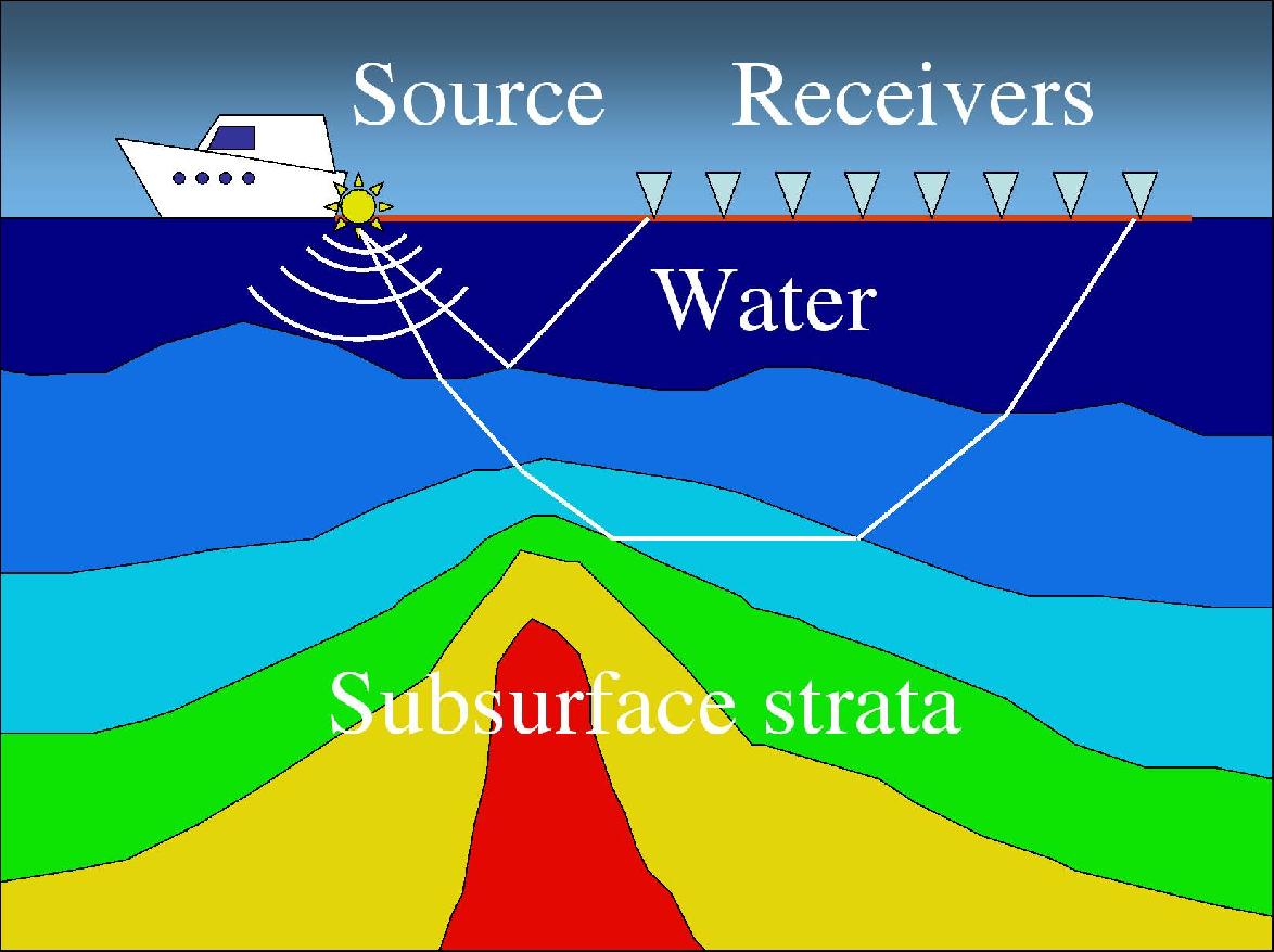
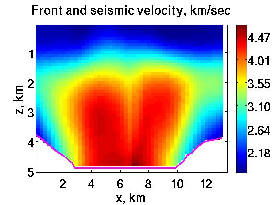
    Imagine a boat releasing impulsive sounds waves (a.k.a. explosions) at equal intervals of time. The pressure waves propagate down to the seabed and then deeper into the earth: they are reflected by both the seabed and from underground layer boundaries. Seismic data are produced by towed receivers which record the amplitudes and times of the reflected signals.

    Our goal is to build a fast and robust algorithm for finding the sound speeds ("seismic velocities") inside the earth from these data. Careful measurements of the seismic velocity are part of obtaining accurate seismic images showing layers and cracks inside the earth, and are used to determine geologic features, such as the location of oil trapped at the sides of a salt dome, shown here by the red color.

    What are some challenges in seismic imaging?

    A location of a point A inside the earth can be described in either of two coordinate systems:
    Depth coordinates, on the left above, give a location of a point A inside the earth in terms of its position on the top and depth below. In contrast, time coordinates, shown on the right, think of each point A under the earth's surface as corresponding to a pair (x0, t0): if you imagine a wave starting at point A, x0 is where it first hits the earth's surface, and t0 is the time when it does so. While it may be counterintuitive, seismic data are most naturally first recorded in time coordinates rather than depth coordinates.

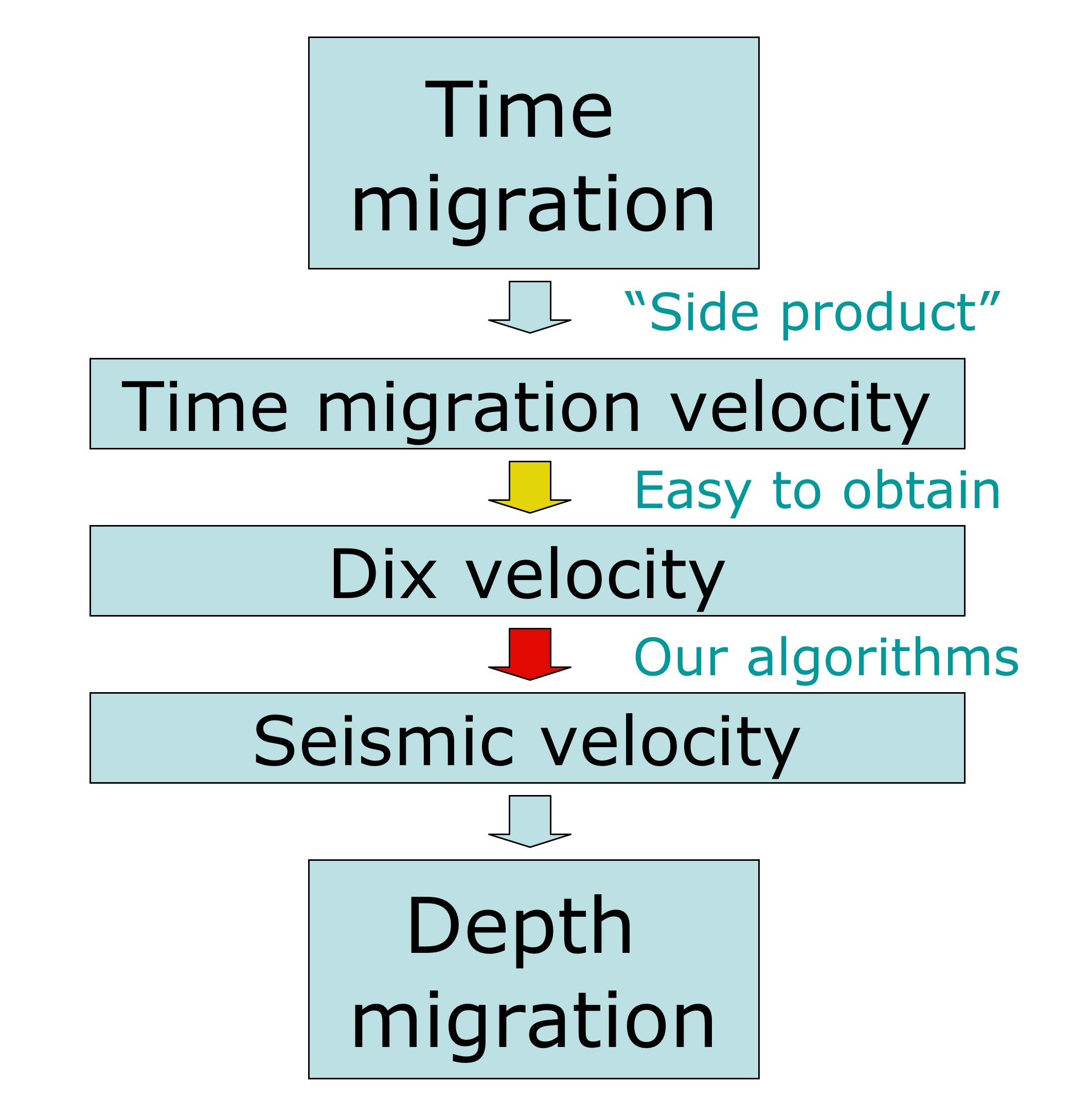
    The two main approaches to seismic imaging produce models for the underground velocities: the first is a process called time migration, which takes seismic data in time coordinates, and produces images and time-migration velocities, which are an averaged velocity of a particular type. The second, depth migration, takes seismic data in depth coordinates and produces seismic images in depth coordinates.

    Time migration has the advantage that it is fast and efficient, however:
    • It works best in areas where the seismic velocity depends only on the depth, in other words, the sound speed is constant along horizontal lines. However, most interesting phenomena, including the presence of underground oil, tend to occur in the areas where flat horizontal structures inside the earth are distorted;
    • Tranforming these images and information from time coordinates to regular Cartesian (depth) coordinates is subtle and non-obvious in cases where the velocity is not horizontally constant and in fact depends on the lateral coordinates.
    In contrast, depth migration produces images in the regular Cartesian coordinates and can be applied when there is considerable lateral distortion in underground structures. However, one needs to start with seismic velocity in depth coordinates in order to apply depth migration: this seismic velocity is never known, and is typically found by "guessing and trying".
     Time migration Depth migration
    Adequate for areas with mild lateral velocity variation arbitrary areas
    Implementation requires nothing seismic velocity
    Produces images in time coordinates depth coordinates

    The inverse problem

    In order to use depth migration, we would like to understand how time migration velocities relate to true seismic velocities in the general case of horizontally variable velocity. If we could accurately transform one to the other, we could exploit the advantages of depth migration in seismic imaging. To do so, we shall make use of an intermediate stage known as "Dix velocities", which relate time migration velocities to seismic velocities in the case of flat horizontal layers, each containing a constant velocity. Sometimes these Dix velocities are directly fed to depth migration codes: one can imagine that this is appropriate when horizonal layers are constant, and hence "time", appropriately scaled, is very close to "depth". However, in the general case of laterally varying layers, this is not particularly accurate.

    Ultimately, we are faced with an inverse problem:

    Numerical algorithms


    We have done the following:
    • First, we have produced a theoretical relation between the time migration velocity and the true seismic velocity in 2D and 3D: we have found that the two are linked through a certain thing called geometrical spreading.
    • Second, we have produced three numerical algorithms for constructing the seismic velocity from the time migration velocity. They are (with some limitations):
      • An efficient, Dijkstra-like time-to-depth conversion algorithm;
      • A conversion algorithm which uses this theoretical relation and a ray tracing approach;
      • A conversion algorithm which uses this theoreticl relation and a level set approach.
    To begin, the first arrival of a propagating pressure wave front can be described by the Eikonal equation. This equation describes when a wave first reaches a point: its right-hand side is the seismic velocity. In our case, this seismic velocity as a function of the depth coordinates (x,z) is unknown, and one of our goals it construct it.
    • Our Time-to-depth conversion algorithm solves the Eikonal equation with an unknown right-hand side: it does this by systematically building the velocity field by coupling the Eikonal equation with an orthogonality relation. Its motivation and a building block was the fast marching method . This algorithm is considerably faster and more robust than existing techniques. However, because we are required to solve two coupled equations simultaneously in order to build the seismic velocity in depth coordinates, a very subtle issue arises as to whether one can maintain causality in systematically building the solution. After an exhausting six months, the answer turns out to be "yes".
    • The Ray Tracing algorithm first solves a system of ray (characteristic) equations for the Eikonal equation as well as the equations for the quantities involved into the relation between the time migration velocity and the seismic velocity. Then the time-to-depth conversion algorithm is used as its final step. This approach is fast, however it fails when the rays start to come too close to each other or spread too strongly.
    • The Level Set algorithm is based on the level set methods . It uses the time-to-depth conversion algorithm as a part of its time loop. This algorithm is slow in comparison with the ray tracing algorithm, but it does not necessarily fail when the rays cross: it follows the "first arrival front".
    We showed on the synthetic data examples that the last two algorithms can significantly improve the accuracy of the found seismic velocity while the conventional approach based on the Dix method can produce qualitatively wrong results. We showed that the problem of constructing the seismic velocity from the Dix velocity is very ill-posed. We used the least square polynomial approximation to suppress the tiny but sharp "bumps" in the seismic velocity under construction.

    Movies of the Algorithms at Work

    Below we show movies of the two algorithms at work:
    Construction of Depth data from Time Coordinates Propagating Interface Filling in Velocity Data

    Synthetic data example

    The exact velocity
    The input data: the Dix velocity
    The found velocity and the rays

    Field data example

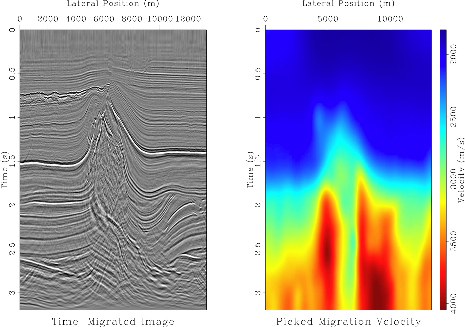
    Left: seismic image from the North Sea obtained by the time migration. Right: the corresponding time migration velocity.

    The image is in the time coordinates. The main feature in it is the salt dome in the middle. Typically, the seismic velocity of the salt is high in comparison with it of the surrounding rock. Note a mess inside the salt dome which indicates that the lateral velocity variation is too severe for the time migration.

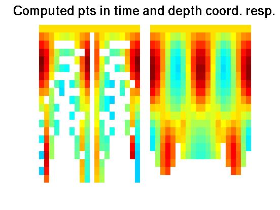
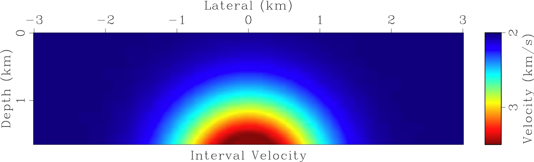
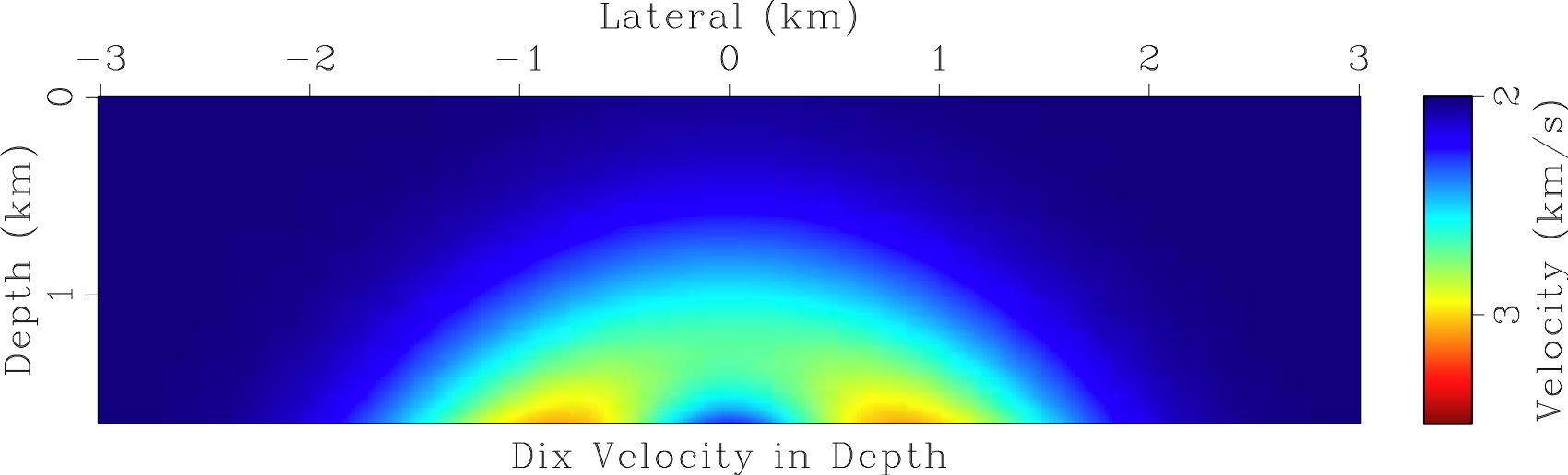
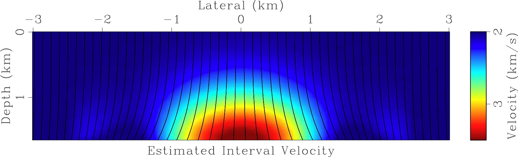
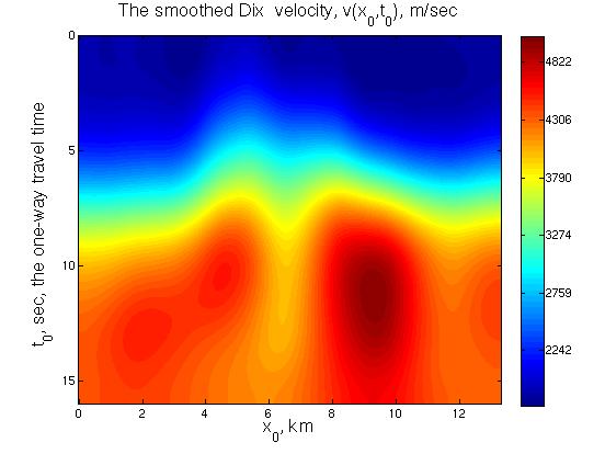
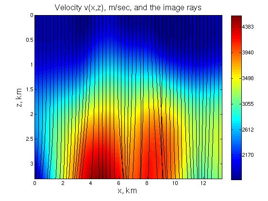
    Left: the input data: the Dix velocity.
    The Dix velocity was obtained from the time migration velocity shown in the figure above and then smoothed.

    Right: the seismic velocity found by our level set algorithm, and the image rays computed for the found velocity. Note that they diverge and intersect and our algorithm successfully handled this. The seismic velocity was cut off at 3.3 km in depth to make the velocity array rectangular.
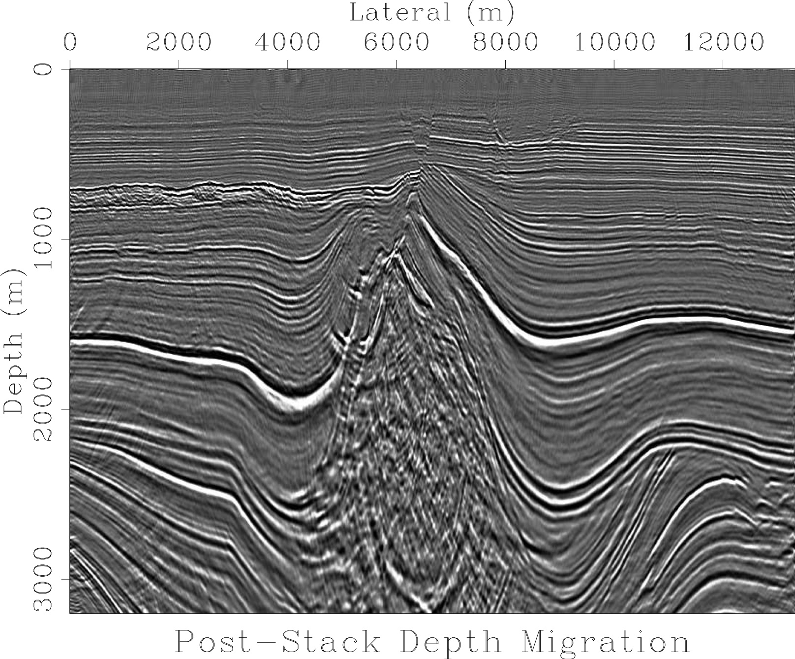
    The depth migrated image of produced using the seismic velocity found by our level set algorithm.
    The image is in the depth (regular Cartesian) coordinates. It is up to 3.3 km in depth which is quite deep according to the geophysical standards. There is a mess inside the salt dome but the surrounding layers are resolved well. Overall, this image looks reasonable.
    References