Investigating the monodromy of the rank-two sheaf microlocal dual to the complex Lagrangian brane $L = \{y = \pm \sqrt{x}\} \subset T^*\mathbb C_x$, we follow the family $hom_{Fuk}(L,T^*_{x = e^{2\pi i t}}\mathbb C)$ of cochain complexes as $t$ goes from $0$ to $1.$ To compute, we turn our heads and consider that $L = \{ x = y^2 \}$ is a graph in $T^*\mathbb C_y,$ and that the family is a family of Morse cochain complexes for the vector fields $\nabla Re ( y^3/3 – ye^{2\pi i t}).$
To follow these around, we must compute the continuation maps. To do so, you track the critical points, but at certain (in this case three) values of $t$ in the family, critical trajectories between same-index critical points appear. These are off-diagonal elements in the parallel transport, contributing with a sign which is determined by the following procedure.
We first orient the ambient $\mathbb R^2$, then choose an orientation of the unstable manifold at each critical point indicated in the picture with a double arrow). This induces an orientation of the stable manifolds such that the product of unstable with stable agrees with the ambient orientation. We then produce a pair of signs from the answers to the following two questions about a critial trajectory from $P$ to $Q$ at time $t=t_0$, where Yes $\Rightarrow +1,$ No $\Rightarrow -1$:
a) Does the trajectory leave with or against the orientation of the unstable manifold at $P$?
b) For $t = t_0 + \epsilon$, does the trajectory deflect away from $Q$ in a direction with or against the orientation of the \emph{stable} manifold at $Q$? (These deviations are drawn in the picture.) The critical trajectory then counts with the product of these signs. At the very end of the loop, we have a matrix organizing the relabeling of critical point, and this is done with signs determined by the compatibility or not with chosen orientations.
This picture summarizes the calculation.
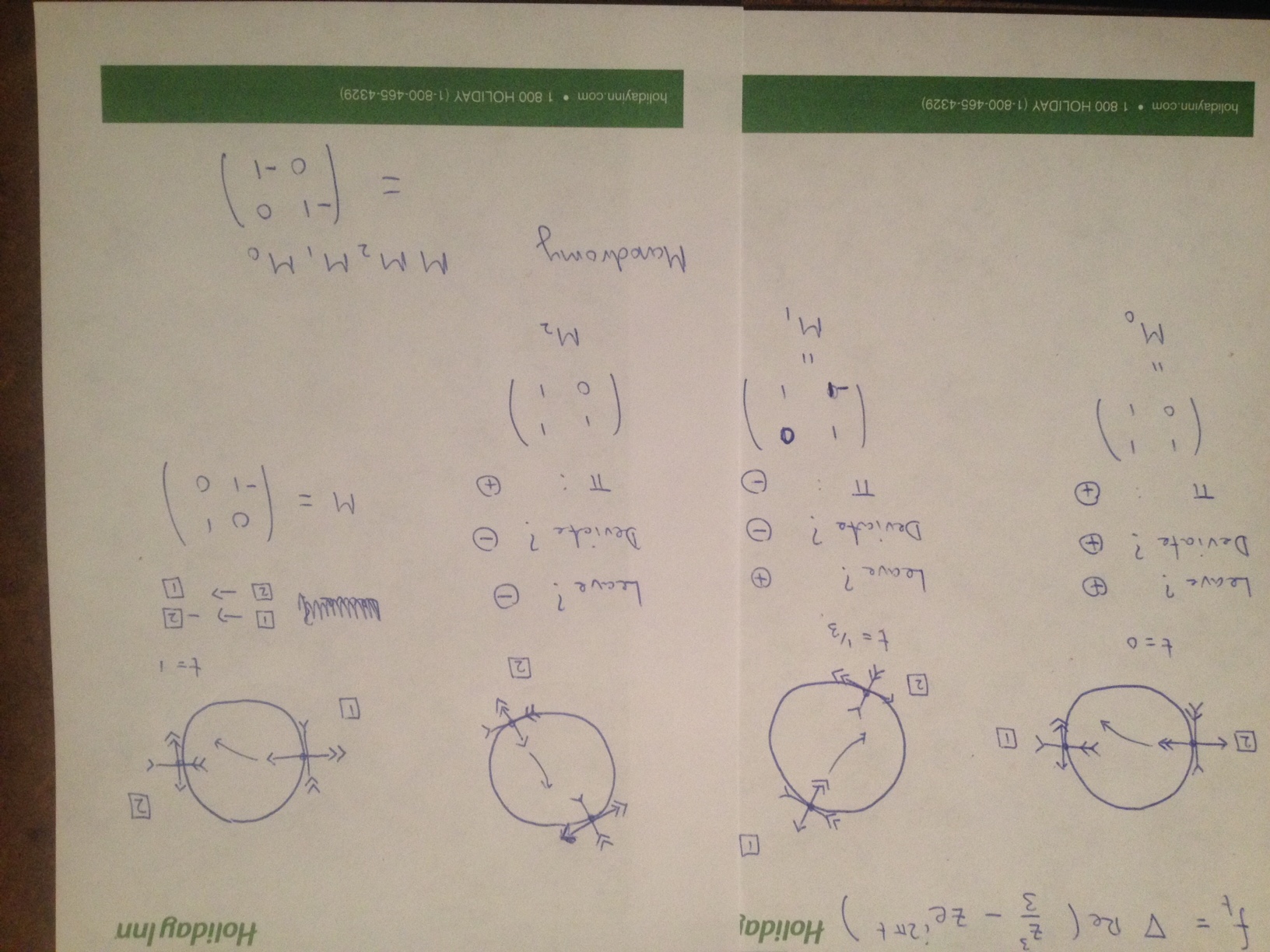
Xin thinks that the monodromy should be $+1,$ and I would have said the same before doing the calculation. Maybe I (and Michael Hutchings, who explained all this to me) made a mistake?
——–
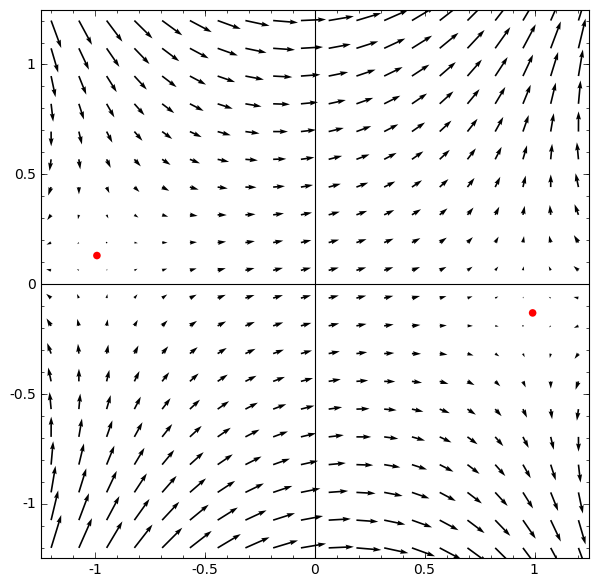
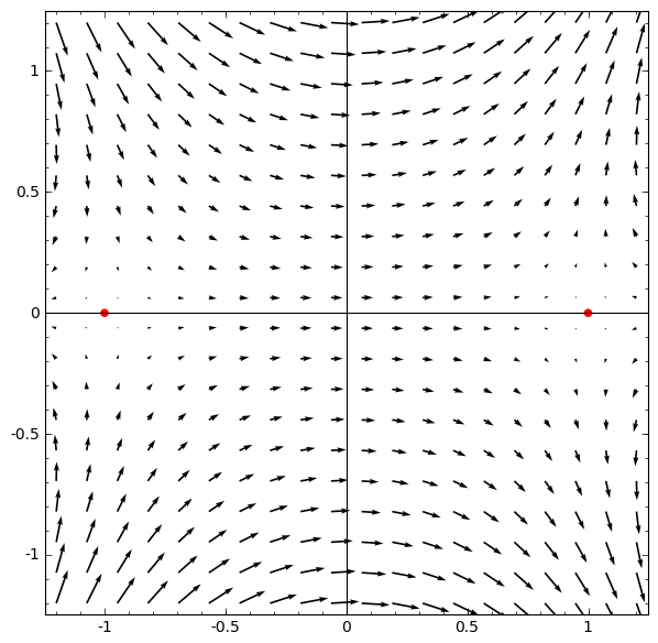
Added 3/16: gradient vector fields for $t = -1/24, t = 0, t = +1/24.$

Hi Eric,
Are the pictures that you drew from images of some software? I just wanted to make sure this part is correct (without reproducing it) and then proceed to check the matrices.
Thanks!
Hi Xin, yes and no. You can derive that the critical points are at $e^{i\pi t}$ and that the stable and unstable axes rotate *clockwise* at half the angle $\pi t$. As for the deviations, it would probably be helpful to draw the vector fields. Here’s a Sage routine that does it.
x,y = var(‘x,y’)
bounds = 1.2
d = [ ]
t = 0
num = 24
for q in range(num):
dnow = plot_vector_field( ( cos(t) – (x^2-y^2) , -(sin(t) – (2*x*y)) ), (x,-bounds,bounds), (y,-bounds,bounds))
dnow += point((cos(t/2),sin(t/2)),size=30,color=’red’)
dnow += point((-cos(t/2),-sin(t/2)),size=30,color=’red’)
d.append(dnow)
t = t + 2*pi/num
for i in range(num):
d[i].show(aspect_ratio=1)
Hi Eric,
Thanks! Can I check one thing? Are the transition matrices $M_i$ from new basis to old basis (i.e. writing coordinates of new basis relative to the old one) or the other way round? From the order of the multiplications, they should be from new basis to old basis. So I guess maybe there is a sign error in the last picture? Because the new basis for the last one is the first picture, and we have $(1)_{new}=(2)_{old}$ and $(2)_{new}=-(1)_{old}$.
Hi Xin, I hope so, but I’ve been over the same argument with myself a few times. Let me make it here.
Let’s start from the left of the page. The critical trajectory goes from basis element 2 to basis element 1. I think of 1 and 2 as column vectors (1,0) and (0,1), so the parallel transport matrix $M_0$ as written correctly indicates where the old basis 1 (at $t = -\epsilon$) arrives under parallel transport in terms of the new basis elements (at $t=+\epsilon$). The monodromy matrix will ultimately tell where the original basis elements (for $t = -\epsilon$) will land in terms of themselves (after rewriting the $t=1-\epsilon$ basis in terms of the $t=-\epsilon$ basis).
Now $M_2M_1M_0 = \begin{pmatrix}0 & 1\\-1&0\end{pmatrix}$, meaning that after going from $t=-\epsilon$ to $t=1-\epsilon$, basis element $1$ (at $t=-\epsilon$) has wound up at the negative of basis element 2 (at $t=1-\epsilon$), which is equal to the negative of original basis element 1 at $t=-\epsilon.$ Similarly, basis element $2$ (at $t=-\epsilon)$ has wound up at basis element 1 at $t=1-\epsilon$, which is negative basis element 1 at $t=-\epsilon.$ So I calculate a monodromy of -1.
Did I make a mistake? I hope so!
One observation is that a reversal of the sign convention for the critical trajectories leads to a monodromy of +1 in the above (still-possibly-incorrect) calculation. I have asked Michael if the opposite convention is perhaps preferred.
I guess the part I was confused about is correct. If we write change of basis from old to new, then the matrices are written from the right to the left.
I cannot run your sage codes correctly, and I haven’t used sage for a long time. Could you post the pictures for $t=\pm\epsilon$? I just wanted to compare your matrix crossing $t=0$ with the matrix using the other way I posted. Thanks!
Well, $M_0$ happens first, and that is on the right, then $M_1,$ etc. I’ll put up some pictures at $t = -\epsilon, t = 0, t = +\epsilon.$
Thanks! I guess the vector field should be $\bar{z}^2-e^{-it}=(x^2-y^2-\cos t, \sin t-2xy))$, so pointing reversely.
Michael confirms that the opposite convention is indeed correct, so the monodromy is +1. Case closed!
Great! I guess the previous matrix is from new basis to old basis.