Effective dynamics for perturbed mKdV

Here is the precise formulation of our theoretical result – see [7, §1].

Let b(x,t) = b₀(hx,ht) where b₀ is a smooth function with bounded derivatives, and h is small.

Let δ > 0 and δ₀ > δ₁ > 0 be any small fixed constants. Suppose that u(x,t) solves (1) with

Then, for

we have

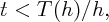
where a(t) and c(t) evolve according to the effective equations of motion,

The time up to which the approximation is valid, T(h)∕h, is given in terms of

where

Under the assumptions on c, T₀(h) > δ₂ > 0, where δ₂ is independent of h

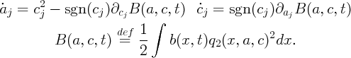
Here is an illustration using the example from the introduction. The blue curve shows the effective motion on top of the black curve showing the solution to the PDE:

For the discussion of the result, see the remarks after the statement of the main theorem in [7, §1.1]. The effective equations of motion (2) have a simple interpretation in terms of Hamiltonian structure – see [7, §1.2].

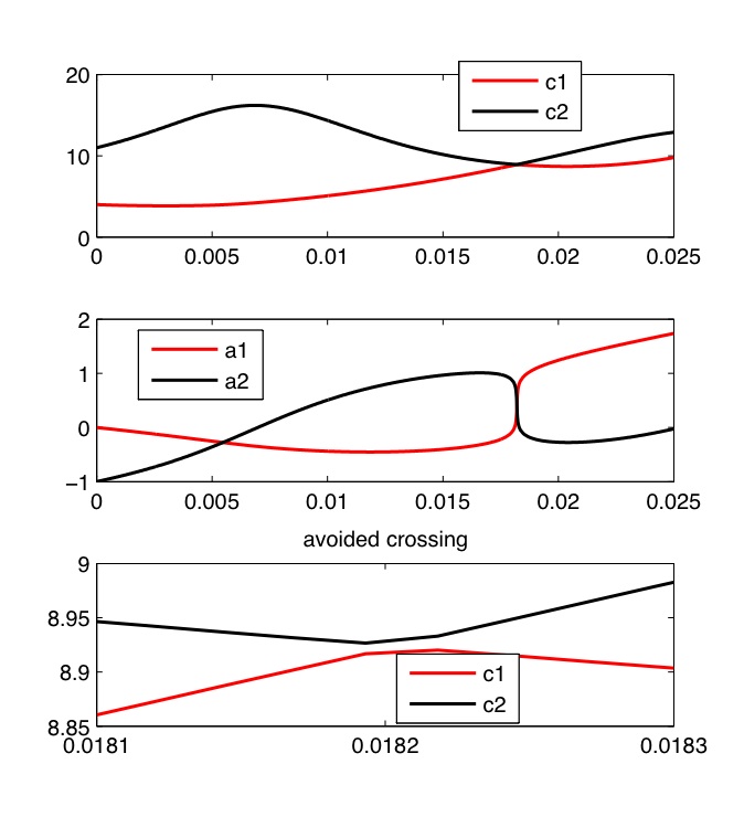
The condition that the velocities of solitons are separated is most likely not necessary (it is violated even at the end of the last movie, yet the agreement with the effective dynamics stays strong) – see the discussion in [7, Appendix B]. The figure below shows the plots of masses and positions of the effective double soliton for the evolution shown above (note the avoided crossing between the red and black curves):

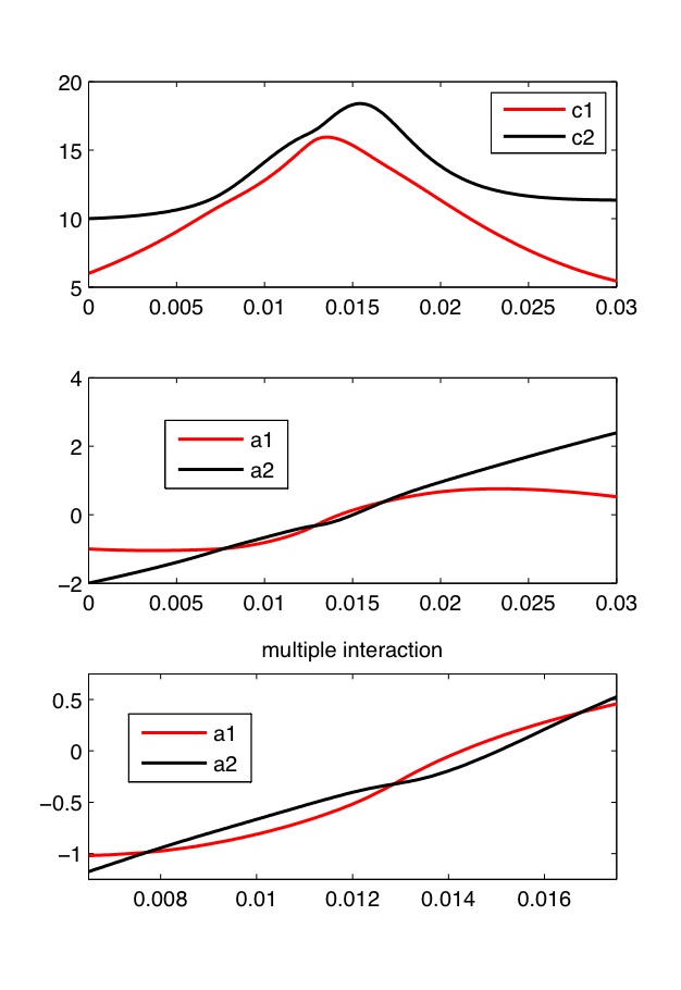
Sometimes we can have multiple interaction of two solitons in the setting allowed by the theorem, that is, without velocities getting close to each to others. Here is an example of an interaction with a Gaussian bump obtained by using the code described in the next section:

The parameters are obtained using another code described in the next section: