MATLAB codes
The code for solving perturbed mKdV: mkdvB.m.
This is a simple adaptation of Nick Trefethen’s code for solving the KdV equation, p27.m. It solves


on [-π,π] with periodic boundary conditions.
mkdvB.m is used as follows:
T = mkdvB(fun,tmax,[a1,a2,c1,c2],N)
where fun represents B(X,T), a function of X and T which should be periodic in x, tmax is the time length; [a1,a2,c1,c2] are the parameters of the initial double soliton; and 2N is the number of grid points (the default value is N = 8, but it may need to be increased for some data).
Here is an example:
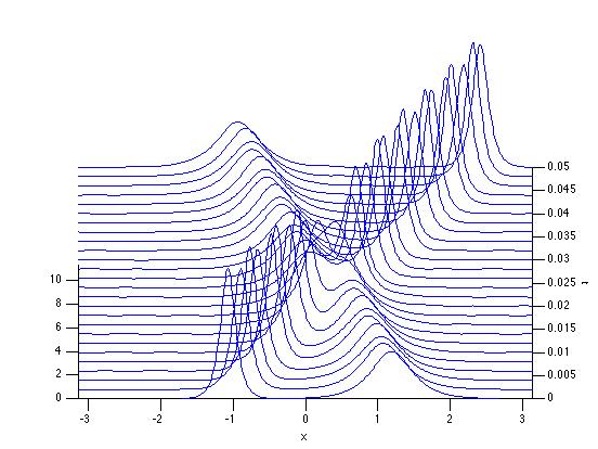
T = mkdvB(@(x,t) 100*cos(x-10^3*t).^2, 0.05, [1,-1,4,11],9)
which returns the following figure
The code for parameters of effective motion: effdyn.m
Here we solve the effective equations of motion (2):
[T,Y] = effdyn(fun,T,[a1,a2,c1,c2])
where fun is a function of x and t which should be periodic in x, T is a vector of time values, and [a1,a2,c1,c2] are the initial conditions. It returns the same time vector and an length(T)-by-4 array of values of [a1(t),a2(t),c1(t),c2(t)], and a figure which can be compared to that returned by mkdvB.m.
Here is an example:
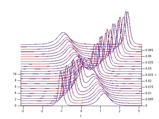
[T,Y] = effdyn(@(x,t) 100*cos(x-10^3*t).^2, T, [1,-1,4,11])
which, when applied with T given by mkdvB.m returns the following figure (new plot in red):
The code for making movies: Bmovie.m
To execute this code effdyn.m must be in the same directory. We use it as follows:
Bmovie(fun,tmax,[a1,a2,c1,c2],N,d)
where the inputs are the same except for the last one: when d = 1 (the default) then the solution of the PDE is shown simultaneously with the solution given by the effective dynamics (the former in black, the latter in blue). Otherwise, only the solution of PDE is shows.
Here is an example:
Bmovie(@(x,t) 100*cos(x-10^3*t).^2, 0.05, [1,-1,4,11],9)
which returns: