Introduction
The modified Korteveg-de Vries equation (mKdV)
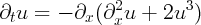
enjoys a multisoliton solution whose explicit form is obtained using the inverse scattering method.
A double soliton q2(x,a1,a2,c1,c2) initial data gives an explicit solution

For ±t ≫ 0, the solution u(x,t) is approximately given by sums of individual solitons of mKdV:
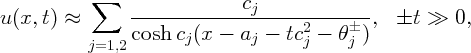
where, for c2 > c1 > 0,
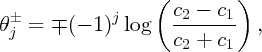
with similar expressions when c1 > c2.
For this and the explicit formula for q2, see [4] and [7, §3].
An example with a1 = 0, a2 = -1, c1 = 4 and c2 = 11 is shown below:
We want to understand the perturbed equation
 | (1) |
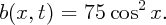
The external potential, b(x,t), is supposed to be slowly varying:

Alternatively, as we do in numerical experiments, we can consider c large:

The properties of b(x,t) in that regime come from simple rescaling (see [7, §1.4]):

Here is an example with the same initial data as above, but with
This movie is obtained using the MATLAB code described below:
Bmovie(@(x,t) 75*cos(x).^2, 0.025, [0,-1,4,11],8,0)
We would like to approximate the solution of (1) with

by

where aj(t)’s and cj(t)’s are solutions to a system of ordinary differential equations.