I want to riff a bit on Vivek’s “microlocal test curves” and in particular try to synthesize it with David’s calculation from earlier in the summer that the trivialization of a cone over a disk looks like a cluster variable. TLDR: monodromy trivialization homotopies are exactly the data of “wrong-way parallel transport” across a negative intersection with a $C_i$.

We expect the coordinate ring $\mathcal{M}(\text{Skeleton})$ to have a basis labeled by $H^1(\Sigma,Z)$ i.e. the “tropical dual” of the cluster torus. As Vivek points out, for classes that pair positively with all the $C_i$ parallel transport along a test curve in that class give the function. If the $C_i$ are a basis, the cohomology classes pairing to +1 with a single curve are the initial cluster variables. Let’s consider the next simplest case, where you have a test curve that has exactly one negative intersection. Again by general theory this is the label of a cluster variable one mutation away from the initial cluster variable, up to a monomial in the other initial cluster variables. Conisder $A_2$ as below, where I label the stalks with different letters for clarity in the subsequent discussion:

Take, say, a curve that goes from right to left across the picture, intersecting the vertical curve and not the horizontal one. How can we associate a function on $\mathcal{M}(\text{Skeleton})$ to this in a geometrically natural way? Well, regardless of whether $y$ is zero or not, the disk attachment means any microlocal sheaf carries a trivialization $y’$ of the monodromy of the cone over $y$:

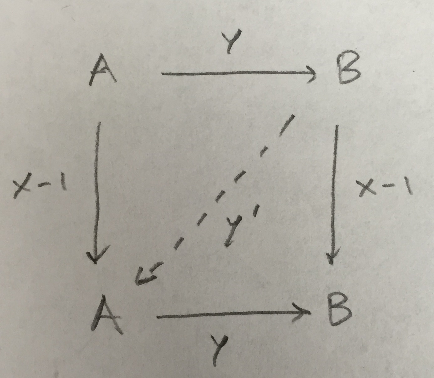
That is, every microlocal sheaf includes the data of a map $y’$ *from $B$ to $A$* that satisfies $yy’ = x – 1$. Which is great, because 1) a map from $B$ to $A$ is exactly the kind of thing that would make sense out of “parallel transport” along the “wrong-way” test curve, and 2) the resulting “parallel transport” is more or less exactly what we expect, a cluster variable:

Of course, the wrong-way parallel transport picture does not naively extend to cluster variables more than one mutation away. For starters, it’s not remotely isotopy invariant. And if you apply it to cluster variables more than one mutation away the naive thing doesn’t get what you want. E.g. in the above example if you consider a curve going from the top right corner to the bottom left, you might naively assign to that test curve the product $x’y’ = (1 + x + y + xy)/xy$ (ignoring signs now). But in fact you want $(1 + x + y)/xy$. Each individual disk tells you e.g. “even though $y$ doesn’t divide 1 in $\mathbb{C}[\mathcal{M}(\text{Skeleton})]$, it does divide $x+1$” and somehow you need to read off from the two disks attached at a point that “even though $xy$ doesn’t divide 1, it divides $x+y+1$”. In some sense there has to be a way of making this explicit and combinatorial, since somehow the combinatorics of quiver Grassmannians and scattering diagrams is necessarily encoded in the kinds of pictures we like to draw…

Also, some of what I said above needs justification from the gradhat picture, for which I appeal to the group. Model the above example with the left gradhat:

Here $Y$ is the cone over $y$ and in both pictures I write the microstalk above right of the given picture (and ignore shifts). I believe that whatever $W$ is in the left picture it essentially has to be the cone over $y’$ (in general, maybe up to a monomial involving the monodromy “in one direction”). I can’t quite get this from the existing description in the blog, which I think is due to my failure to interpret the term “global sections” in a sufficiently homotopical sense.