Ideal Webs and Exact Lagrangians

October 30, 2014

Let me recall what an ideal web is, then throw out a partially-baked question regarding their relationship to exact Lagrangians. The notion of ideal web appears in unpublished work of Goncharov (see here: http://people.math.umass.edu/~tevelev/AGNES_vids/Goncharov.mp4), but builds on a lot of pictures familiar from earlier work of e.g. Postnikov and relates those pictures to his work with Fock.

—-

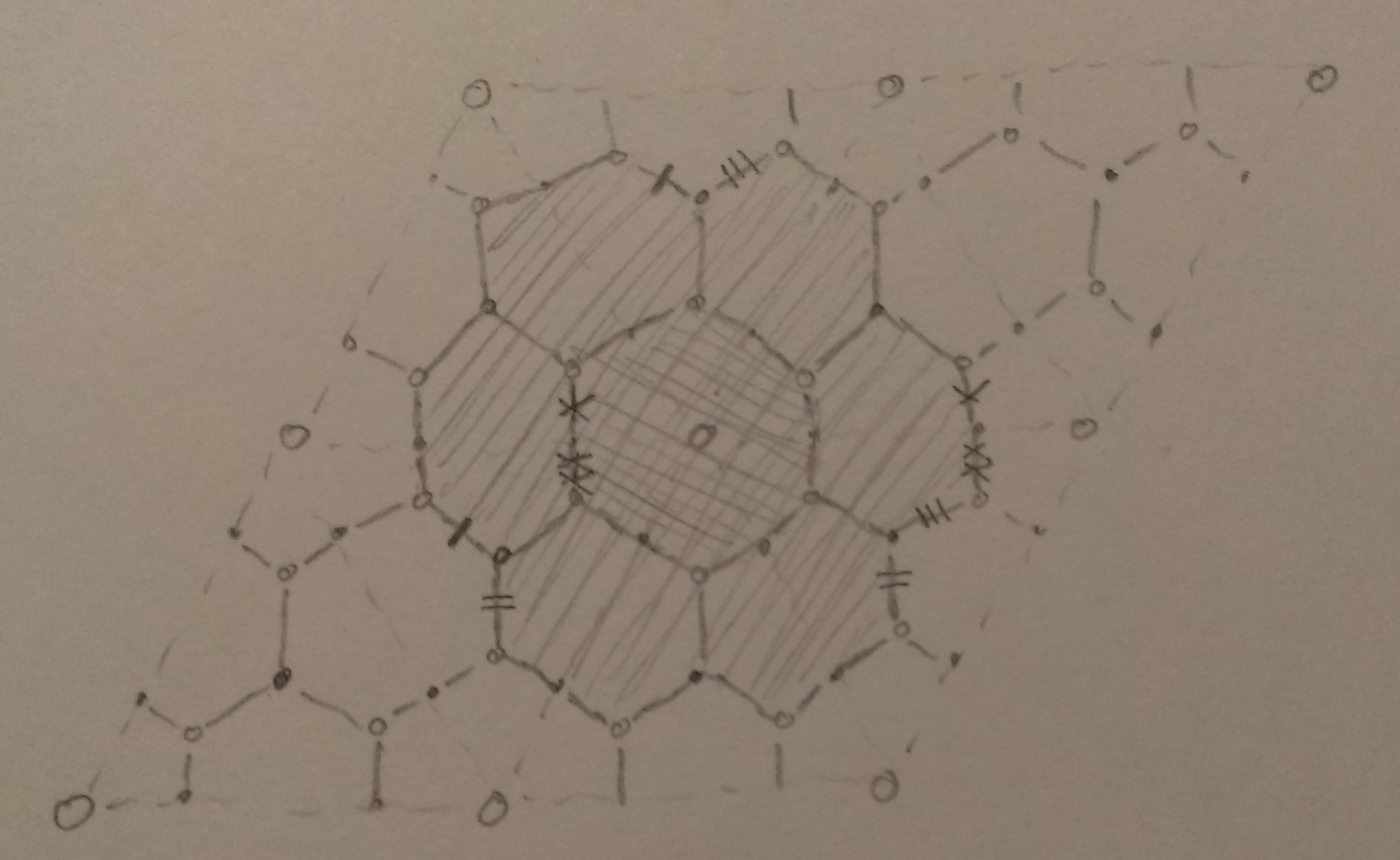
First let me recall a standard story. The starting point is a bipartite graph $G$ embedded into a marked surface $S$ (maybe with marked points on a boundary). The basic examples are of the following form: pick an ideal triangulation of the surface, then built a bipartite graph out of local models like the following:

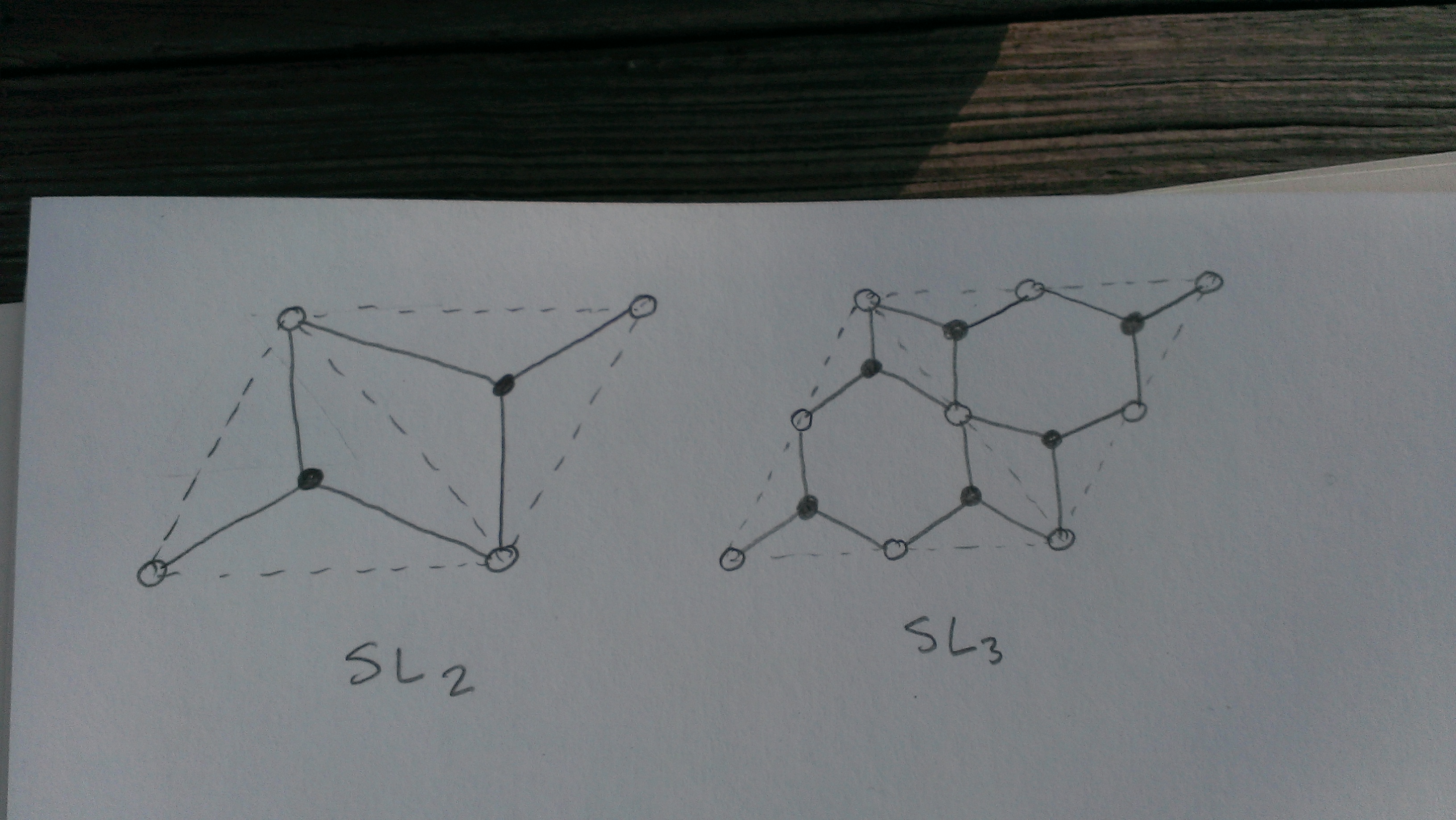
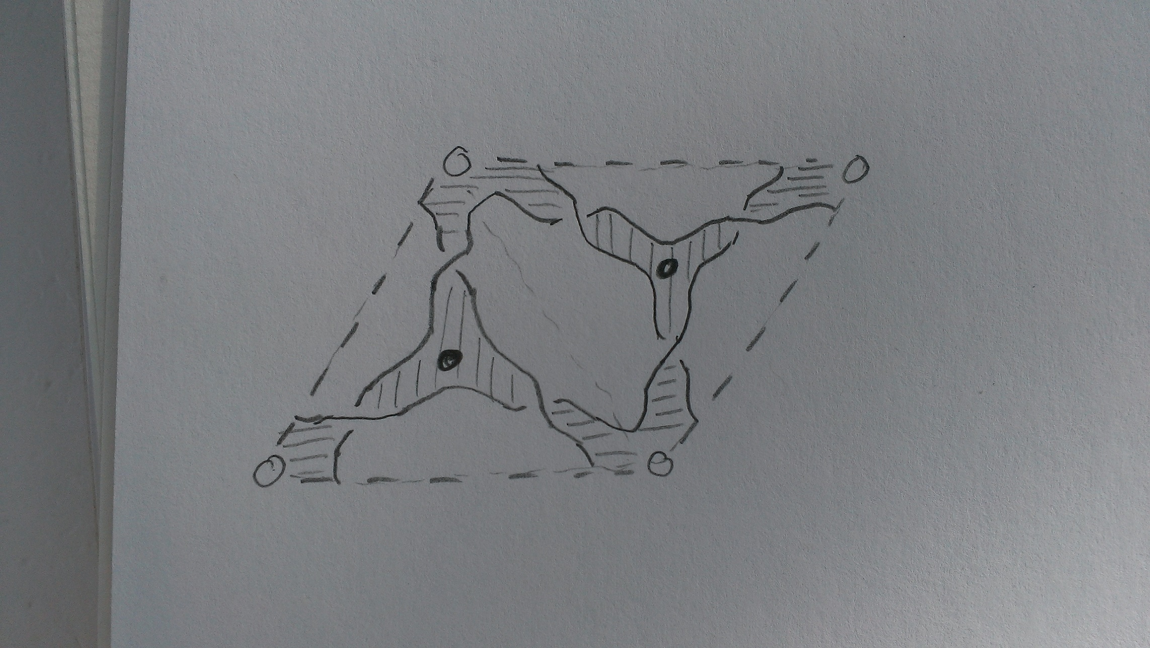
Note that every marked point is the location of a white vertex, and every black vertex is trivalent (there’s a $G L$ version he draws in the video). From $G$ we build a surface $C$ , called the conjugate surface of $G$ : take the ribbon graph which is a tubular neighborhood of $G \subset S$ , and insert a half-twist along each edge. This projects to $S$ and its image looks like:

$C$ comes with a homology basis given by faces of $G$ in $S$ . These coordinates identify the space of $G L_{1}$ -connections on $C$ with the cluster torus built by Fock-Goncharov.

—-

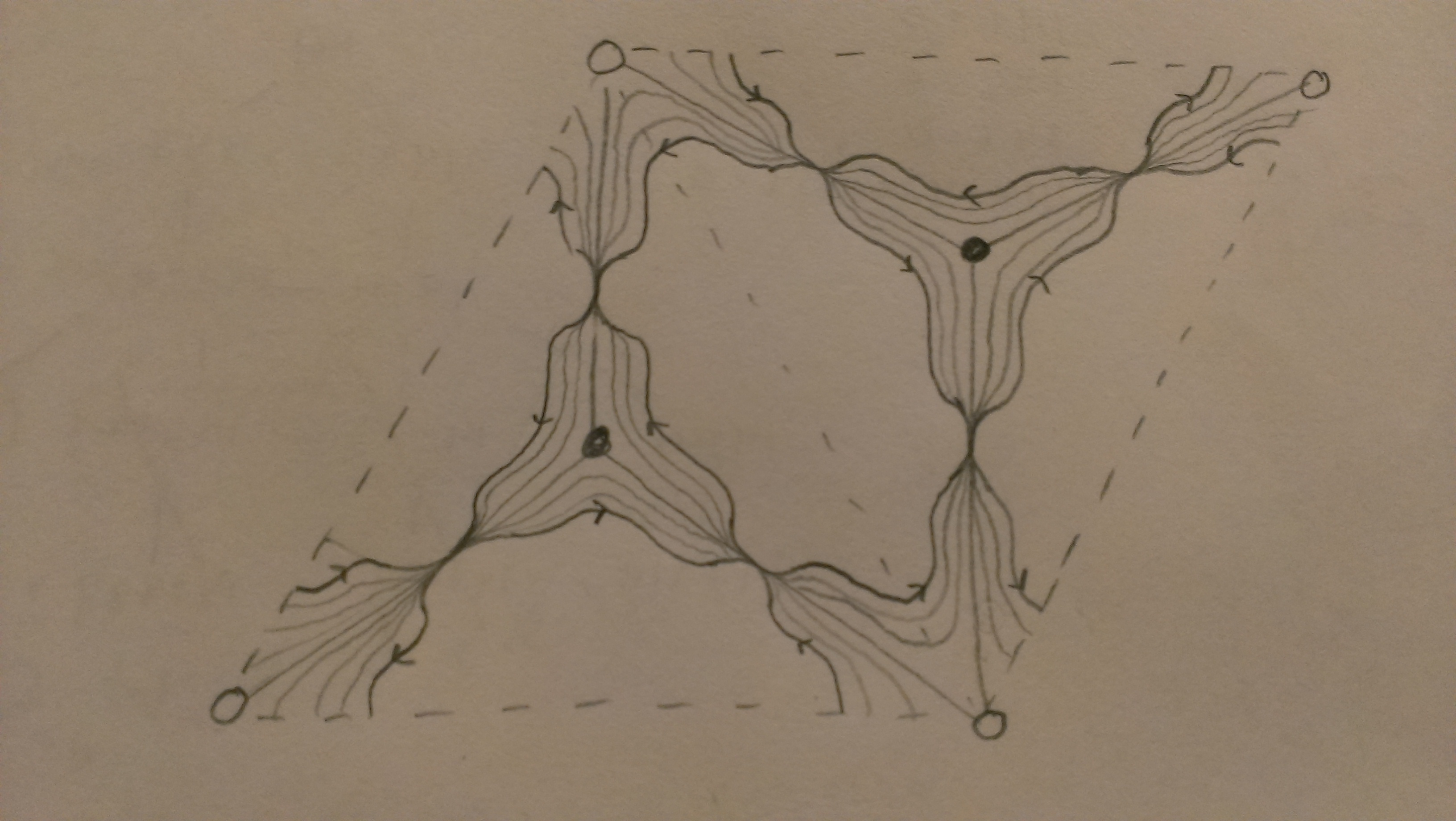
Here’s Goncharov’s story. The conjugate surface can be “stretched out” into a branched cover, which can be identified topologically with a spectral curve of the corresponding Hitchin system (see 37:30 in the video). We can build this branched cover directly from the bipartite graph: the point is to glue together a bunch of (possibly punctured) disks, each of which is glued out of all faces touching a particular white vertex (he phrases it slightly differently, but I think it’s the same). Here’s a picture for the punctured torus: we take the shaded disk in the universal cover, and there’s a unique way to glue it up so that the resulting surface is a 2-sheeted cover branched at the black vertices:

Now one feature of this construction is it gives a recipe for deforming the spectral curve (as a topological surface mapping to $S$ ) so that it exactly covers its image in $S$ , except at the half-twists. From the point of view of knots, I imagine this can be described as follows. We start with some knot projections drawn around the punctures on the base surface (so the data defining a knotty character variety), and we drag the strands of those projections around the surface so that their intersections satisfy some combinatorial conditions (in Goncharov’s language, they form an ideal web, i.e. they arise as the projections to $S$ of the boundary of the conjugate surface of a bipartite graph). From the point of view of STZ, I would expect these combinatorial conditions are equivalent to “constructible sheaves with singular support on the original knot diagram which are of rank n away from the punctures (i.e. wild rank-n local systems) are equivalent to constructible sheaves with singular support on the ideal web but whose stalks only ever have rank 1 or 0.” In discussions with Vivek and Eric earlier in the semester we’d drawn a similar picture relating the ruled surface you guys associate with a braid diagram to the conjugate surface of an associated bipartite graph: you sort of “pull down” some edges of the ruled surface and you get the conjugate surface. But after talking with Vivek it clicked that Goncharov’s construction gives a different perspective on this as well as a wide generalization.

—-

And now to the point: I’m told by my betters that building exact Lagrangians ending on knots is not so easy. But maybe the above train of ideas means we can instead worry about building exact Lagrangians ending on ideal webs, and naively that seems a lot simpler. With respect to the ideal web, the constructible sheaves we care about are rather simple: they are rank 1 in a bunch of combinatorially described patches and 0 elsewhere. So a naïve person would think building an exact Lagrangian corresponding to this sheaf should also be simple (since higher rank stalks are out of the picture), along the lines of playing some game with d log of a bump function supported on the rank 1 patches. There is something nuanced that happens above the half-twists, but at least this is a uniform local picture one only has to figure out once. If that’s doable, then it would be pretty natural to conjecture something like: inverse microlocalization applied to this canonical exact Lagrangian ending on an ideal web recovers the cluster chart associated by Goncharov/Fock-Goncharov to that ideal web.

—-

A perhaps superfluous remark: we can take half-twists as the local picture, but they can also be “sucked in” to the black vertices, being replaced by a different local picture:

I don’t know which is preferable from the point of view of building exact Lagrangians.

—-

Another notion Goncharov introduces is the distinction between ideal webs and a more general thing he calls spectral webs: basically ideal webs satisfy a minimality condition the more general spectral webs do not, and are exactly the spectral webs corresponding to honest character varieties. I don’t think he discusses these in the video I linked, but during the talk I saw I asked what the geometric meaning of the more general webs was and he said he didn’t know one. I bet we do: they correspond to general knotty character varieties.

—-

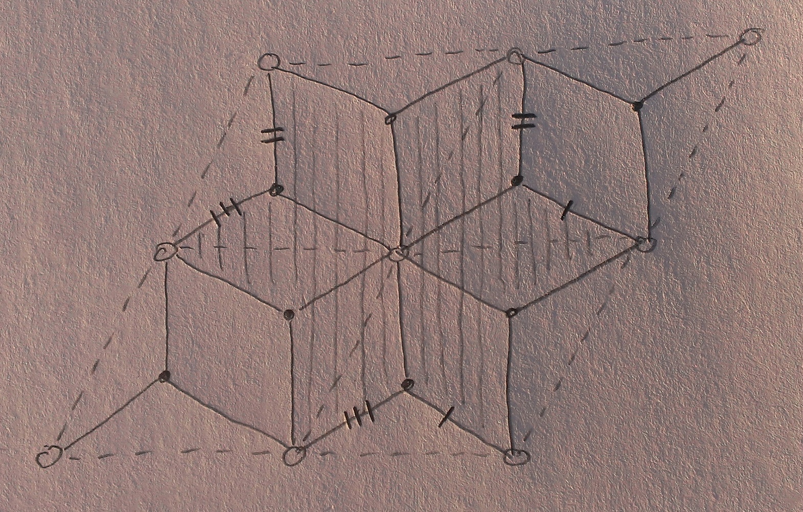
$G L_{2}$ spectral cover for the once-punctured torus, glued out of 2 punctured disks in its universal cover:

—-

Added 11/7/14:

Let me first address the issue of one of these pictures “only being part of the spectral cover”. I would disagree and instead say the following: to an ideal web are associated two surfaces with different combinatorial constructions, but which turn out to be homeomorphic. They are both built out of pieces of $S$ , so come with canonical maps to $S$ , but these maps are very different in nature. One is the conjugate surface: it is built by taking a tubular neighborhood of the bipartite graph, then gluing in a half twist in the middle of each edge. It comes with a canonical map to $S$ which is injective except at the middle of the half-twist. The other is the spectral cover: it is built by gluing together several possibly-punctured disks corresponding to zig-zag paths in the graph. Each such disk is the bounded component of “the universal cover of $S$ minus a lift of a particular zig-zag path”. It comes with a canonical map to $S$ which is a branched cover.

So I would not say it’s true that the conjugate surface is “only part of the spectral cover” and that you get the spectral cover by “filling in the disks corresponding to the zigzag paths” (sorry if I am just totally misunderstanding you).

—-

Here is a more detailed version of the construction I’m proposing. I’m going to try to associate an exact Lagrangian $L$ to a bipartite graph/ideal web. It will be obviously identified with the conjugate surface $C$ in a way that commutes with their respective maps to $S$ . Here are the steps in the construction of $L$ :

1. First, choose paths on $S$ representing the strands of the ideal web (i.e. the zig-zag paths). I’ll draw them so that at each crossing the two strands are tangent to the bipartite graph $G$ (maybe this isn’t necessary, but makes it easier for me to convince myself that $L$ is doing what I want it to at the half-twist).

2. Let $U \subset S$ be the interior of the image of $C$ . It is a union of (possibly punctured) disks each containing a unique vertex of $G$ .

2. Let $f : U \to [- 1, 0) \cup (0, 1]$ be a smooth function which

a. takes values in $(0, 1]$ (resp. $[- 1, 0)$ ) on disks containing a black (resp. white) vertex,

b. is equal to $\pm 1$ on $G$ ,

c. extends to a smooth function on $\overset{―}{U} ∖ (G \cap \partial U)$ equal to 0 on $\partial U ∖ (G \cap \partial U)$ .

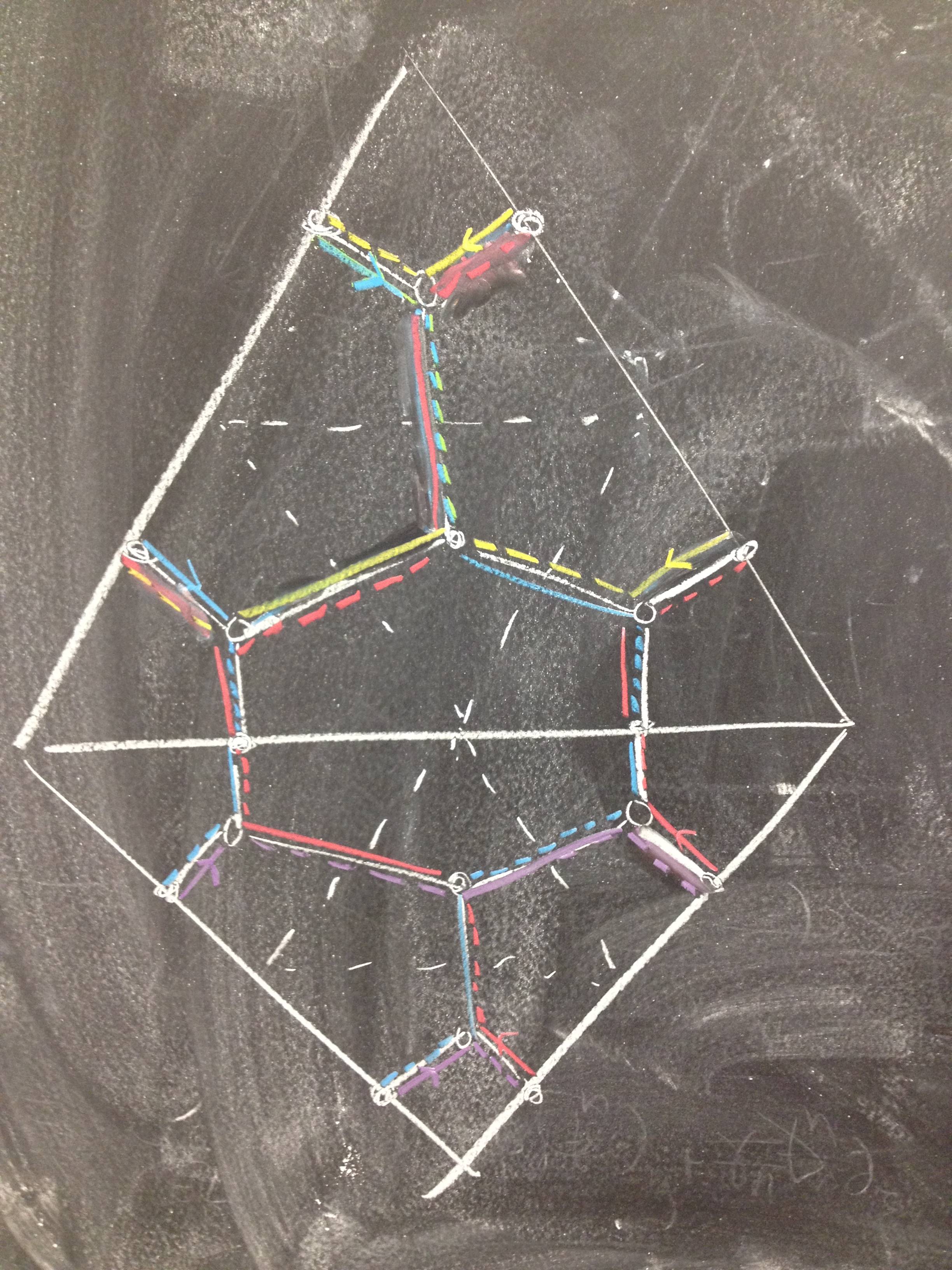
Here’s another a detailed picture of the $S L_{2}$ once-punctured torus case, where I have drawn in some level curves of such a function:

3. $L$ is the closure in $T^{*} S$ of the image of $d \log f$ . The complement in $L$ of the image of $d \log f$ is composed of a line in the cotangent space of each crossing of the ideal web. Each such line is the set of covectors killing the tangent direction to $G$ .

I think I’ve set things up so that $L$ is a smooth exact Lagrangian but correct me if I’m wrong.

Conjecture. The cluster chart of the ideal web is the inverse microlocalization of $L$ .

What do you guys think?

—-

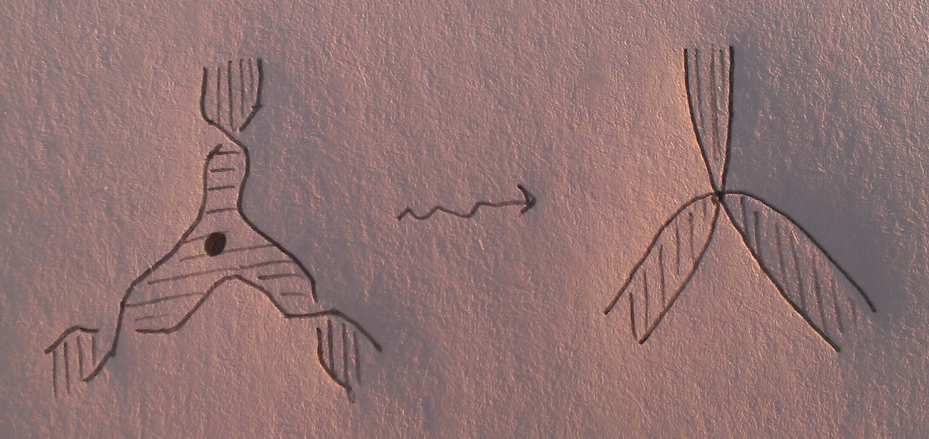
Here is a local question that sounds like something you guys would have thought about. It involves the local picture of “twisting” the conjugate surface to create a branch point. On the upper level of the picture below, let’s call the surface on the left $C_{0}$ and the one on the right $C_{1}$ :

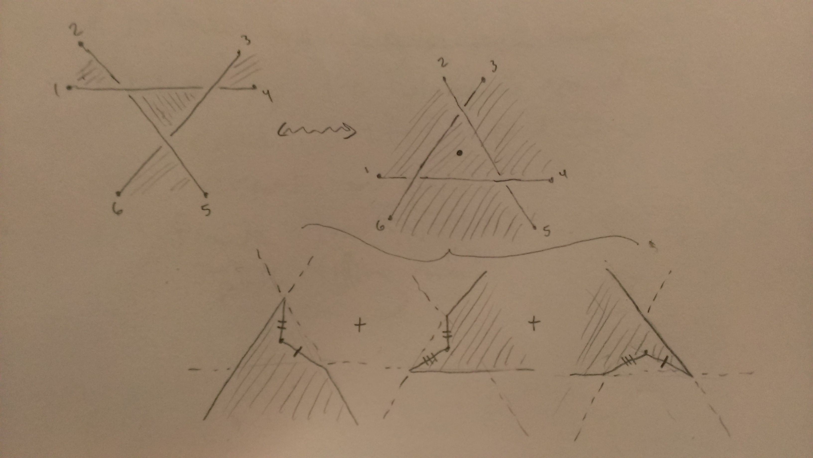
I’ve drawn each with a projection onto the page, the surface $C_{1}$ being a 2-1 cover in its central region as pictured. There is an oriented homeomorphism between $C_{0}$ and $C_{1}$ which at the boundary of each picture commutes with their projections to the page (i.e. takes points 1-6 on $C_{0}$ to the corresponding points on $C_{1}$ ) . However, when I imagine both surfaces sitting above the page in $R^{3}$ , it doesn’t seem like there is an isotopy between them in $R^{3}$ that is constant at the boundary of each picture (i.e. fixes points 1-6).

Question. If I take both surfaces to be sitting above the page in $R^{4}$ , is there an isotopy between them in $R^{4}$ that is constant at the boundary of each picture?

The fact that the conjugate surface and the spectral cover are homeomorphic is just a computation of their genus and number of boundary components. But I would hope that given the embedding of the conjugate surface into $T^{*} S$ , they would actually be isotopic. So this is a local version of that global question.

———

Zaz including photo here:

——

HW 11/11:

——-

HW 11/11:

45 comments

October 30, 2014 at 10:24 pm

davidtreumann says:

This is terrific. Does the conjugate surface already come with a preferred embedding into the cotangent of the base?

I’ve encountered the sheaves on these local models before, e.g. page 5 of arxiv:1010.4071. If you straighten out the curved lines in the “sucked in” picture, you get a conic sheaf whose Fourier transform is the constant sheaf on the union of three rays from the origin. So one option for a Lagrangian in the cotangent of the ideal triangle is to thicken this trivalent vertex to a open set, take $d \log (m)$ , and regard the cotangent coordinates as coordinates on the triangle.

Reply
- October 31, 2014 at 1:23 pm
  
  Harold Williams says:
  
  It’s definitely not typical to view it with a preferred embedding into $T^{*}$ , but it certainly seems like it should given our discussion.
  
  Can I clarify the relationship between degrees and orientation: looking at your reference, it seems that if I pull apart the sucked in picture, I’m really supposed to be thinking about rank 1 sheaves whose stalks in the inner region (the one with the black vertex in my picture, the light triangle in yours) are shifted by a degree from the stalks in the 3 regions on the other side of the half-twists. From the point of view of the conjugate surface, the two types of regions are distinguished by whether the projection from the conjugate surface to the base is orientation-preserving or orientation-reversing. So I’d think that degree shift has something to do with how our Lagrangian is supposed to be oriented — is this correct, and is it a point you understand clearly?
  
  Reply
  - October 31, 2014 at 2:39 pm
    
    ericzaslow says:
    
    I haven’t followed the discussion enough to comment, but degree (of a sheaf corresponding to a Lagrangian) has to do with the winding of Lagrangian tangent planes in the ambient symplectic tangent bundle. In the case of a folding sheet of a surface where you can fix one tangent vector to be constant, you basically have the winding of the slope of a line in the circle of possible angles.
    
    Reply
    - October 31, 2014 at 3:02 pm
      
      haroldwilliams says:
      
      Ahh ok, that at least makes me less confused mod 2. Let me add another remark which seems germane to orientation issues. The strands in the ideal web have a canonical orientation by the rule “as you cross an edge, a black vertex is on your right” (rather there are two canonical orientations, this one and its reverse).
      
      Reply
November 1, 2014 at 6:43 am

ericzaslow says:

Harold, are your pictures slightly different from Goncharov’s? His m=2 has more vertices interior to each triangle. Is this the difference between SL and GL that you mention? Also, for Goncharov m is the number of zig-zag paths surrounding a face. In your illustration there are 3 (if they are all distinct). Is this due to the difference between SL_3 and GL_2 as well?

Reply
- November 1, 2014 at 1:13 pm
  
  haroldwilliams says:
  
  That’s right: see for example 51:14 where he draws an $S L_{3}$ picture.
  
  I think if $m$ is the number of zig-zags surrounding a face then the group is either $G L_{m}$ or $S L_{m + 1}$ , and he just wasn’t more specific since at that point in the talk he had only drawn $G L$ pictures. For example, I added at the end of the post a drawing of the $G L_{2}$ spectral cover of the once-punctured torus, to complement the $S L_{2}$ picture further up. For $S L_{2}$ there is actually just 1 strand in the ideal web, whereas for $G L_{2}$ there are 2. In the pictures of the disks in the universal cover I just smushed the strands up against the edges of the bipartite graph to make the picture less busy. And doing the exercise one see that you produce the same surface, just the $G L_{2}$ web constructs it as a gluing of 2 disks and the $S L_{2}$ web constructs it as a gluing of 1 disk.
  
  Reply
November 7, 2014 at 8:35 am

ericzaslow says:

Hi all. The zigzag paths are the boundary components of the conjugated ribbon graph, so you just fill those in with the corresponding disks. To model them as sheaves/Lagrangians, I propose the following. Take a black Y vertex. Each of the three v-shaped parts of it corresponds to a region of the local neighborhood containing 2/3 of the picture (not 1/3). We want to put a sheaf in that region. Consider the following rule, meant to mock the twist of a ribbon graph. For the part of the “v” corresponding to the zigzag entering the black vertex, put standard boundary conditions, and for the part exiting, put costandard. Take the sum of these three sheaves. This is a generically-rank-two sheaf. Now since standards meet costandards on edges, the corresponding Lagrangians will intersect, and we are going to want to take the surgery over the intersection. This will remove the singularity at infinity and create a single, double-sheeted Lagrangian cover (except we don’t know what it does at the origin). I guess in the end this is just $\sqrt{z} d z$ .

Reply
- November 7, 2014 at 3:08 pm
  
  ericzaslow says:
  
  After chatting with David, I guess I should point out explicitly that Harold’s picture only represents the part of the conjugated surface (=spectral cover), i.e. before filling in the disks corresponding to the zigzag paths. Once you do that, you get the m-fold cover over the original surface. My point was that one should be able to build from this data a sheaf whose corresponding Lagrangian is the spectral cover. To go beyond my comment above, which was just local to a vertex, do the following: take the disk interior to a zig-zag path and give it alternating standard and costandard boundary conditions (alternating at each edge), with the convention (say) that when you exit a black vertex in the direction of orientation you do so with standard boundary conditions. Then standards will always (at least as far as I’ve checked) abut costandards, and this should allow us to glue. But sheaf-theoretically, you don’t have to glue, you can just take the formal cone (if you like). (Confession: around a Y in $\bR^{2}$ , I know how to do this by looking at the unit circle. I guess you can extend to R^2 minus a point and then push forward, but I haven’t thought about how to do this more globally on the Riemann surface — but it doesn’t seem complicated.)
  
  [I can’t make pictures at the moment.]
  
  Reply
  - November 7, 2014 at 11:56 pm
    
    haroldwilliams says:
    
    It sounds like you are describing something different than what I was trying to propose, so maybe I will try to restate what I was advocating more precisely. Indeed, part of the idea was to never touch a multi-sheeted Lagrangian cover directly. I added my comment to the end of the post so I could include a picture.
    
    PS: Can I really not add pictures to comments? Or do I just have to know what I’m doing?
    
    Reply
    - November 8, 2014 at 1:54 pm
      
      haroldwilliams says:
      
      So thinking about it more I’m worried that the Lagrangian $L$ is not exact because of what’s happening at the half-twists. If that’s the case let me rephrase the question as: can we do something else along these lines to embed the conjugate surface into $T^{*} S$ as an exact Lagrangian in a way that commutes with its projection to $S$ ? And then does inverse microlocalization of that Lagrangian recover the cluster chart?
      
      Reply
      - November 8, 2014 at 2:12 pm
        
        ericzaslow says:
        
        It looks to me as though your picture would be the same as my comment at 8:35AM on Nov. 7 if you just looked in the central triangle region. I think you wanted to use sheaves in lieu of the Lagrangian cover, and what I proposed (at 8:35AM) was a concrete sheaf model for this part of the cover and (at 3:08PM) for the rest of the surface, too. In order for my sheaves to line up and glue the way you indicated, I needed to impose opposite boundary conditions for the sheaves on either side of a glued edge. (It is not clear to me why you do not consider the rest of the spectral cover, i.e. just the thickened twisted ribbon graph is not enough, as its boundary components have not been filled in: that’s what the disks are for.)
        
        After thinking a bit more, I think that what I described for the unit circle in $R^{2}$ (for the case of a single Y vertex) can be extended more generally. Namely, for each polygonal region (the disk inside a zigzag path), put a sheaf on a hub-and-spokes shape. (So if the region were a square, start with a sheaf on a + sign.) Give the endpoints of the spokes the appropriate boundary conditions. Then the polygonal region \emph{minus the vertices} retracts to the hub-and-spoke, so we can pull back the sheaf we had built to the whole polygonal region minus the vertices. Then we will glue by taking a cone over the morphisms that exist (but, say, don’t do the geometric surgery if you don’t want to) along edges.
        
        Reply
      - November 8, 2014 at 2:47 pm
        
        haroldwilliams says:
        
        One quick question before I parse this more fully: what does it mean that the conjugate surface is “not enough, as its boundary components have not been filled in”? In the embedding into $T^{*} S$ it is a closed Lagrangian submanifold, and sure its boundary lives at infinity, but what of it? We’re supposed to be trafficking in noncompact Lagrangians, right? Are you saying the conjecture as I phrased it is false, or that there is a technical reason why it is not well-posed?
        
        BTW I’m not sure why it wouldnt let me reply to eric’s comment directly, but this is in reference to his comment on 11/8 at 2:12pm.
        
        Reply
        
        November 8, 2014 at 3:24 pm
        
        ericzaslow says:
        
        Hi Harold, maybe I don’t understand the picture well enough. I see a ribbon graph. Where do the edges of your ribbon live? They are real codimension one boundary components. If they live at infinity, then why are we considering them rather than the spectral curve that Goncharov defined, which is constructed by gluing in disks which bound the edges of these ribbons?
        
        Reply
      - November 9, 2014 at 12:53 am
        
        haroldwilliams says:
        
        Ah ok, I think I’m just not so adept in the sheafy language yet, so got confused easily, but am starting to understand you better. I had left my last discussion with Vivek with the following impression, tell me if this is correct: Suppose we have a knotty character variety, defined by a bunch of knot projections drawn around the punctures of $S$ , and we drag the strands of the knot projection around the surface until they form an ideal web (maybe there are some local rules governing the type of dragging we allow). Then it’s essentially a result you guys already have that the knotty character variety (let’s call it $M_{k n o t}$ ), a particular space of sheaves constructible with respect to the knot projection, is isomorphic with a space of sheaves constructible with respect to the ideal web (let’s call it $M_{w e b}$ ). Of course, I have tell you which sheaves, in particular what ranks they should be and where, but this can be extracted from STZ. And $M_{w e b}$ has the property that the stalks are all rank $\leq 1$ . Is that all correct? And were your comments spelling out this isomorphism more?
        
        If that is correct, the reason I am using the conjugate surface rather than the spectral cover is that I thought the basic narrative of what we wanted to do was the following: we want to apply $μ^{- 1}$ to an exact Lagrangian and get a toric chart on $M_{k n o t}$ , and show that this toric chart coincides with a cluster chart. But we don’t know how to actually produce an explicit exact Lagrangian that does this, though clearly it should be a relative of a Hitchin spectral curve. So I was saying “instead look at the Lagrangian $L$ , which is not a branched cover but is explicit and $μ^{- 1}$ applied to it gives a toric chart on $M_{w e b}$ . Then compose this with the isomorphism $M_{w e b} ≅ M_{k n o t}$ , and we get a toric chart on $M_{k n o t}$ which hopefully is the cluster chart.”
        
        So I was taking this iso $M_{w e b} ≅ M_{k n o t}$ for granted, and you should tell me whether that’s really appropriate.
        
        Reply
November 9, 2014 at 7:08 am

ericzaslow says:

I think we need Vivek and David to chime in, because I’m getting out of my league here.

Let’s just consider a disk with a single singularity. Then we know that $M_{k n o t}$ is isomorphic to a space of connections with a fixed singularity type, and this has a spectral curve description, too.

What do you mean by $M_{w e b},$ since I have never heard of sheaves constructible with respect to the real codimension one stratification produced by a web? Instead I think of the large cells of this stratification as charts for Sol, the local system which is the sheaf of sections, the Stokes data being gluing data for these sections. These sheaves have rank m for GL_m.

So I don’t know what is meant by $M_{w e b}$ here, sorry.

That’s how I read paragraph one. But if I try to continue…

“If that is correct, the reason I am using the conjugate surface rather than the spectral cover”

Is your “conjugate surface” just the ribbon part of a surface, and not what you get when you fill in the boundary components? I would say that when you fill its boundary components in you get the spectral curve.

Anyway, the narrative in my head (rather, what I thought you were originally espousing — maybe this morphed into my own narrative) is to produce those rank-m pieces over the triangulation — i.e. the strata where Sol is trivialized — and these will correspond to m different rank-one sheaves on those strata, i.e. m different exact Lagrangian graphs. The tricky part, then, is to determine the gluing data for these sheaves. I had been proposing boundary conditions which would ensure that neighboring sheaves had a morphism between them, over which we could take the formal cone and build a sheaf whose corrsponding Lagrangian — even if we couldn’t write it down — is the sought-after spectral cover.

But maybe I’m confused enough that we should try to organize a video chat.

Reply
November 9, 2014 at 10:31 am

David says:

Hi Harold. Can you check my work in one example? I don’t have time to create a picture but I can tell you some statistics of the thing I drew, and you tell me if it passes the smell test.

Start with a base surface S, which is just a disk. Distinguish 5 points on the boundary of S, and an ideal triangulation of S with 3 triangles.

I drew what I think is the “GL2 web” in each triangle. The bipartite graph has 9 white vertices and 17 black vertices in all. 10 of those black vertices are leaves.

When drawing the conjugate surface, I’m not sure what to do with the leaf vertices. The options I like are: omitting them, or drawing a loop around them. In either case the conjugate surface I draw has one boundary component (snaking all over the place on my drawing).

Regarding that boundary component as a Legendrian knot, should I hope it’s isotopic to the (2,5) knot whose front projection is supported close to the boundary of S?

Reply
November 9, 2014 at 10:37 am

ericzaslow says:

David explained Harold’s idea to me. Let me try to recapitulate. If we, say, begin with an ideal triangulation of a decorated, closed surface (I don’t really understand the nonclosed case — see below), then there will be m zigzags for each vertex of the ideal triangulation. We then “push off” the zigzags to create immersed curves for each path. Interpreting the picture of the immersed curves as front projections of Legendrians, we get Legendrians in $T^{\infty}$ of the surface. We could 1) isotope those curves to a neighborhood of their corresponding marked point to get some Legendrian data near those marked points and an equivalent associated category. Or, we could 2) leave them alone and try to build a microlocal rank one sheaf with singular support in the Legendrian at infinity.

Harold wants to do (2) *and* have the Lagrangian and the corresponding sheaf both supported in a vicinity of the bipartite graph. I was trying to do (2) but create a spectral cover from the data. So Harold’s sheaf would be generically rank 0, and rank 1 near the bipartite graph, while mine would be generically rank m. That explains the difference in our approaches, and I hope clarifies the misunderstanding!

Later comes the question about what to do with marked points on the boundary, probably corresponding to Stokes rays. David suggests that if the zigzags go around the edge of the surface then they can curl back in and ultimate have some interesting knotting.

Reply
November 9, 2014 at 2:56 pm

ericzaslow says:

Running with Harold’s original interpretation (as I now understand it), a local model for where the twist happens at an edge (oriented vertically, say) is given by an X shape with microlocal hair pointing in some directions. I’d guess that *before* the twist it points always inward to the edge, corresponding to standard sheaves in north and south regions, but *after* twisting we get standard in south and shifted-costandard in north (or vice versa). So we have a standard thickened Y around each black vertex and a shifted costandard thickened Y around each white vertex? Then there is a degree-one hom (ext) at the midpoint of each edge and the final answer should be determined by the choice of extension class over each edge.

Reply
November 10, 2014 at 10:47 am

ericzaslow says:

I put in a photo of zigzag paths with some standard (solid line) and costandard (dashed) indications., but I’m not presuming to know what it means. It’s a nice photo, though.

Reply
November 10, 2014 at 11:11 pm

Harold Williams says:

Hey guys, sorry for being AWOL yesterday, I had a bunch of pressing things come up.

RE 11/9 10:37: Awesome, yes, I think that was exactly the misunderstanding!

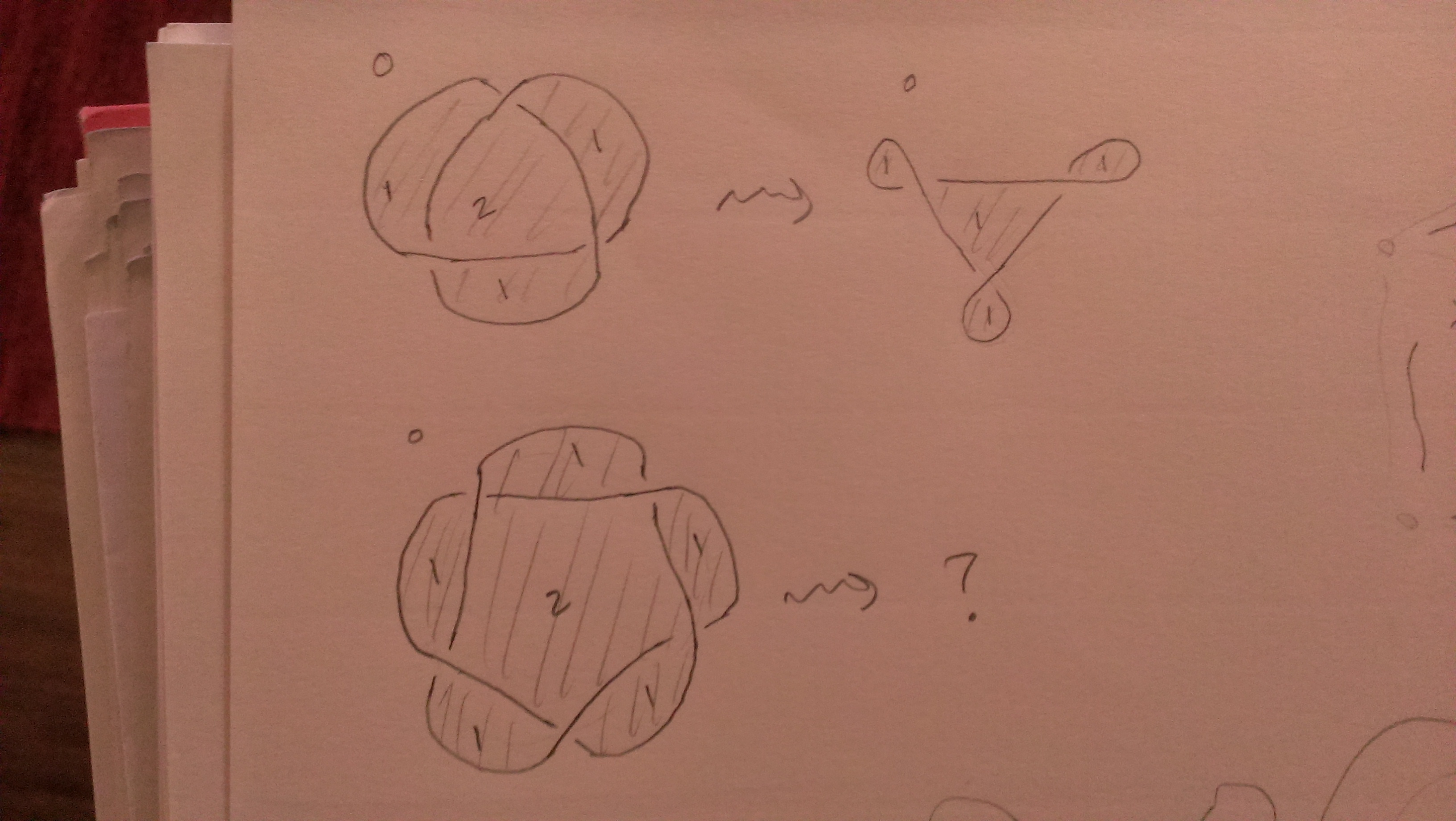
RE Marked boundary points: I must admit I don’t really know how this is supposed to work — Goncharov mentions this topological doubling procedure, but that looks weird from our point of view. It seems like in the example David mentions, we do want things to be related at the end of the day to a (2,5) at infinity. I wonder if it’s enlightening to try to work backwards. That is, rather than start with the picture of the ideal web where we don’t quite know what to do with the boundary, let’s start with the picture of the (2,5) knot and try to play with it and its moduli space of sheaves until we get a new picture with an equivalent moduli space of sheaves of rank $\leq 1$ . And hopefully we recover the “right” picture of what we’re supposed to do with the triangulation. I attached a picture of a late-night partial attempt at this, but I need to go to sleep so I will just post it and hope it makes some kind of sense.

RE “So we have a standard thickened Y around each black vertex and a shifted costandard thickened Y around each white vertex?”: I don’t really know the standard/costandard language yet, so I’ll ask the first in the series of a million stupid questions (I read the definition in NZ, but don’t have the right pictures in my head yet). Suppose I have a Lagrangian $L \subset T^{*} X$ corresponding to the standard sheaf over some $Y \subset X$ . Does $- L$ correspond to the costandard sheaf over $Y$ ? Sorry if the question doesn’t make sense, I’m just trying to get a feel for how your statement relates to the picture I had of the Lagrangian $L$ I mentioned above.

Reply
- November 11, 2014 at 1:12 am
  
  David says:
  
  Suppose I have a Lagrangian $L \subset T^{*} X$ corresponding to the standard sheaf over some $Y \subset X$ . Does $- L$ correspond to the costandard sheaf over $Y$ ? Sorry if the question doesn’t make sense
  
  The question makes perfect sense when $Y \subset X$ is open, in which case the answer is “yes.”
  
  Reply
  - November 11, 2014 at 6:06 am
    
    ericzaslow says:
    
    I think I wrote what I did about the X and the Y to try to match the local picture from David’s Klyachko paper. The statement reflects no a priori understanding of why there wouldn’t instead be mixed boundary conditions on north and south. In short, I don’t *really* know how to handle the twist except *somehow* flipping boundary conditions. David?
    
    Reply
    - November 11, 2014 at 1:05 pm
      
      haroldwilliams says:
      
      @ David: Awesome, thanks!
      @ Eric: Those boundary conditions are the ones compatible with the Lagrangian $L$ , the (interior of the) conjugate surface embedded into $T^{*} S$ , “turning over” at the half-twist, right?
      
      Also, can you guys confirm whether the $L$ I wrote down is actually exact, given its behavior at the half-twist?
      
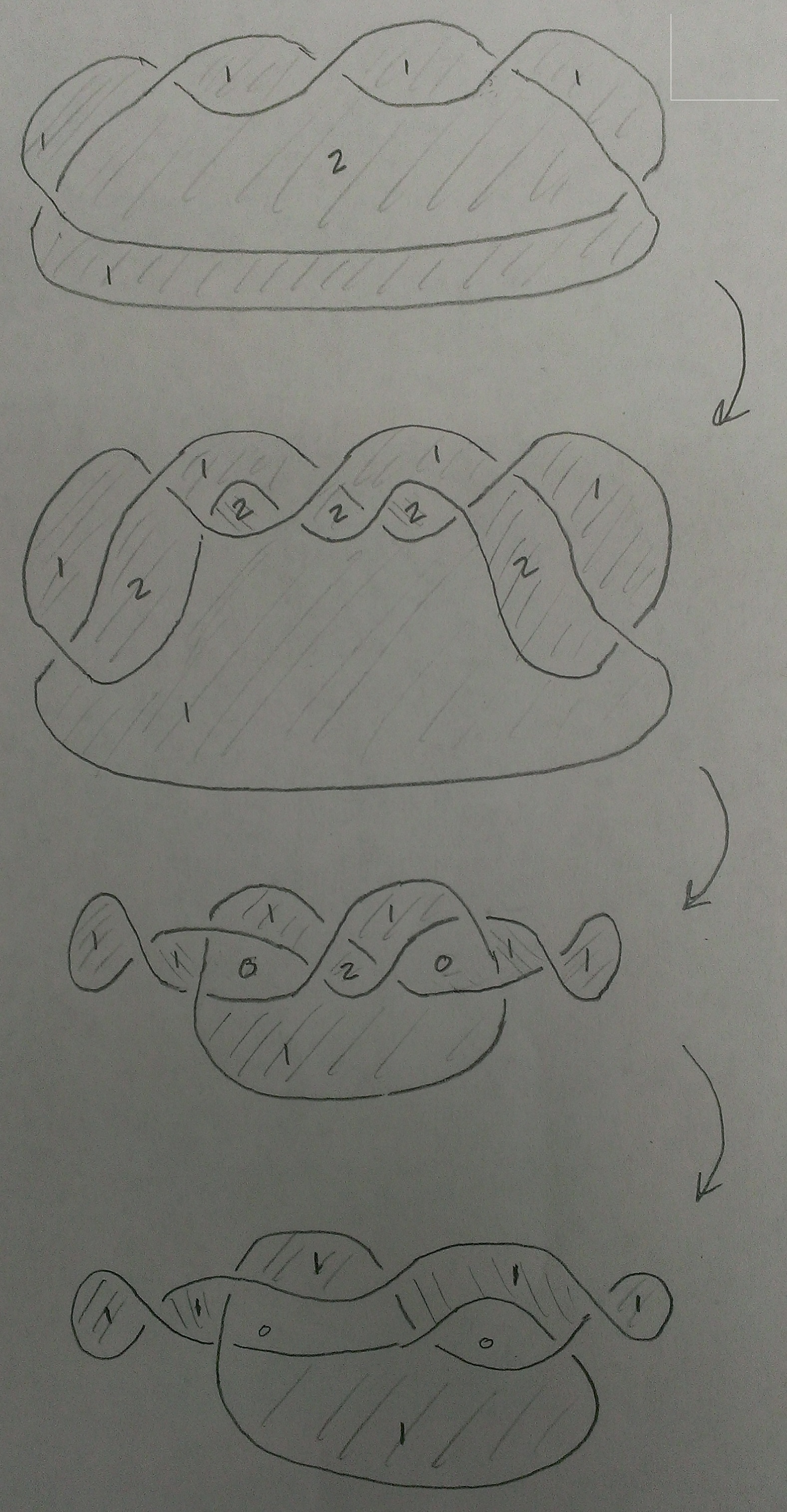
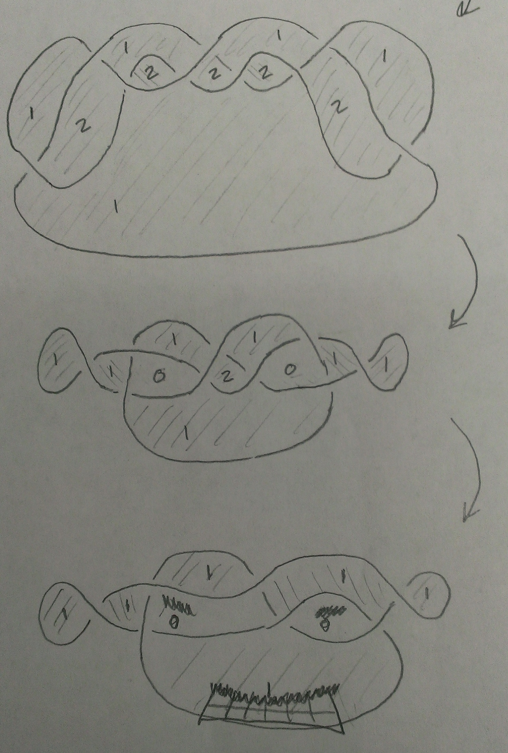
      I also drew more of the (2,5) picture I had in mind last night. I.e. a sequence of moves that starts with the (2,5) and takes it to a configuration whose moduli space consists of sheaves of rank $\leq 1$ . At least, on some formal level it seems right, but I didn’t really think about the boundary conditions, just wrote in ranks of stalks and guessed about the right way to manipulate them. I was trying to bootstrap from the local model of black vertices twisting up into branch points, but in the second picture I just threw in 0’s in the indicated region because it seemed to make the picture work — I don’t know if that’s actually what is supposed to happen with the Reidemeister 2 I introduced there. The final picture is very close to what you get from the triangulation, in particular it has two face cycles. But it also only has two “ears”, which seems funny — does the presence of the ears actually change the moduli space, or can they be removed? I also added a second version where the last picture is drawn as an angry water buffalo. I leave the mathematical significance of this up for discussion.
      
      Reply
      - November 11, 2014 at 1:09 pm
        
        haroldwilliams says:
        
        (Actually I originally put in 2’s there on the second level and then changed them to 0’s in the third — I’m hoping there’s some sense in which they should be 0’s in the second level.)
        
        Reply
      - November 12, 2014 at 1:36 am
        
        David says:
        
        Harold your water-buffalo pictures are enticing, but they don’t fit into the framework of “Legendrian Reidemeister moves for front projections.” So I am scratching my head a little, not sure what I’m looking at.
        
        The ears are not completely innocuous, but they might not change the moduli space. They wind around the circle fibers of $T^{\infty} S$ in a way that looks like it can’t be undone by an isotopy. But maybe it can be undone by a mapping class of $T^{\infty} S$ .
        
        Also, can you guys confirm whether the L I wrote down is actually exact, given its behavior at the half-twist?
        
        I lost track of the conversation and edits. Can you point again to what L you wrote down?
        
        Reply
      - November 12, 2014 at 7:07 am
        
        haroldwilliams says:
        
        Can you point again to what L you wrote down?
        Sure, see the second section of “Added 11/7/14” above — it was meant to be the conjugate surface embedded into $T^{*} S$ as an exact Lagrangian.
        
        Reply
      - November 12, 2014 at 3:25 pm
        
        David says:
        
        Harold your water-buffalo pictures are enticing, but they don’t fit into the framework of “Legendrian Reidemeister moves for front projections.” So I am scratching my head a little, not sure what I’m looking at.
        
        I didn’t notice until now that these sheaves are isotopic to each other. I’m still not sure what to do with the ears, but the (2,5) knot in this picture is coming in to focus.
        
        Reply
November 12, 2014 at 8:41 am

ericzaslow says:

Hi Harold, your $f$ has some nice features but there are some subtleties we have to consider carefully. Your regions meet in cusps rather than corners — locally something like $y^{2} < x^{4}$ rather than $y^{2} < x^{2}$ . Do the corresponding sheaves still have a morphism? If so, then we still, in order to build a finite Lagrangian, need a local model for the surgery over this morphism, and this is already difficult in the $y^{2} < x^{2}$ case. I have been thinking about that case, but still haven't figured out how to do the cone/surgery and present it as a graph.

Reply
- November 12, 2014 at 3:30 pm
  
  haroldwilliams says:
  
  Hmm well the cusp was just something I pulled out of my ass — I thought it made the picture at the half-twist simpler, but if not I have no particular motivation for it. But it sounds like to parse your answer I need to fix some basic misunderstanding I have: my cartoon understanding of part 1 of the game we’re playing is “build an exact Lagrangian which meets $T^{\infty} S$ along the lifts of the ideal web”. So if you’re saying we need to do something more subtle than just looking at the $f$ and $L$ I proposed, is it because:
  1) “Building an exact Lagrangian isn’t enough, it needs to satisfy conditions X and Y which are not obviously satisfied. So even though $L$ is exact we may have to modify it in some way to meet these conditions.”
  2) “ $L$ isn’t actually exact on the nose because of its behavior at the half-twist. So we need to modify it in some way to really be exact.”
  
  Reply
November 12, 2014 at 6:04 pm

ericzaslow says:

I’m saying that your f is not defined at the crossing point (it has to be both 1 and 0 and -1 at the same time, and as a result, your L is perfectly nice away from the crossing but goes to infinity at (over) the crossing. So really you have a bunch of pieces of a would-be connected L. Those pieces meet at infinity, over the crossing. In order to build a single, compact L we need a way to resolve these singularities. If you look at the sheaves corresponding to the pieces of your L, they have morphisms between them living at the crossing. I think we’ll want to take the cone over these morphisms. I say this because in Lagrangian world, taking that cone should bring the intersection at infinity into finite space and resolve it all at once. This is your L as I interpret it.

So how to make that L? Even with the |y| < |x| region I don't yet know — at least not how to put the corresponding L into graph form — and I think it is related to a host of subtle questions that have plagued David, Vivek and I for a long time, and continue to plague me. That said, I haven't thought about this problem in its purely Lagrangian formulation. So that might be a nice thing to try to do….

Reply
- November 12, 2014 at 6:52 pm
  
  haroldwilliams says:
  
  Wait, okay maybe this is why the cusp seemed like a good idea: The picture in my head was that $L$ is $\pm d \log f$ except directly above the crossing $c$ , and the intersection $L \cap T_{c}^{*} S$ is the subspace of covectors that are conormal to the bipartite graph. What the cusp picture had convinced me of was that this is actually is a closed surface embedded in $L$ . This is because if I look at the level sets of $\log f$ near the crossing they are becoming tangent to the bipartite graph. So if I follow a level curve and look at what $d \log f$ is doing, it is approaching a covector which is conormal to the graph. But this is true for $- d \log f$ too, so the two sides “agree” on what $L \cap T_{c}^{*} S$ should be. Is this incorrect?
  
  In the event that it actually is correct, what I did not know was whether $L$ was actually exact above the crossing, given that as you say that the function $f$ doesn’t extend there.
  
  Reply
  - November 12, 2014 at 11:32 pm
    
    David says:
    
    I think I understand $L$ now. It’s great!
    
    You’ve mentioned “behavior at a half-twist” a few times as a possible obstruction to the exactness of $L$ , but I don’t think it can cause any problems. Every Lagrangian is locally exact, for the same reason that every closed one-form is locally exact. Especially, every Lagrangian is exact over a contractible region, such as a half-twist.
    
    Still I’m not sure if $L$ is exact. You’ve constructed it as the graph of a one-form that you call dlog(f), but since f takes negative values log(f) is sort of fictional, the one-form is df/f. Is this one-form exact? I’d like to integrate it around a loop in your picture here to find out, but it got complicated when I tried.
    
    Reply
    - November 13, 2014 at 1:07 am
      
      David says:
      
      Actually, can we change the definition of $L$ ? You propose to change the sign of $f$ according to whether you’re close to a white or black vertex, but $d f / f$ is not sensitive to that sign. Instead we could take $f$ to be positive everywhere and put the sign directly in the definition of the Lagrangian, $L = \pm d f / f$ .
      
      Reply
November 12, 2014 at 9:19 pm

ericzaslow says:

Yes, they agree and they are both infinite. Without a cusp they would occupy an arc at infinity but agree at some point.

Reply
- November 12, 2014 at 9:31 pm
  
  haroldwilliams says:
  
  RE “they are both infinite.”
  
  Sorry is that an agreement or disagreement with my claim about what $L \capT_{c}^{*} S$ is? Or more precisely, if I let $L^{0}$ be the graph of $d \log f$ , what is the intersection of the closure of $L^{0}$ and $T_{c}^{*} S$ ? At the very least it includes $0 \in T_{c}^{*} S$ , right? Because $L^{0}$ contains the bipartite graph itself, embedded into the $0$ -section.
  
  Reply
November 13, 2014 at 6:13 am

ericzaslow says:

To make this concrete, take $f = x^{4} - y^{2} = (x^{2} - y) (x^{2} + y)$ in the right half-plane, and then $d l o g f = (2 x d x - d y) / f + (2 x d x + d y) / f,$ which goes to infinity along the upper and lower parabolas and at the origin is indeed only two rays, up and down. If on the left halfplane you use $1 / f$ then this will accomplish the switch as you desire (when you take the closure). As you have anticipated, since there is no `excess intersection’ near the switch there are no infinities to remove — so that seems pretty good! (I hadn’t realized this feature about the cusp versus the cross, sorry.)

I want to check your $f$ near the vertex. It is a positive function which is supposed to be differentiable and goes to a max of 1 near three spokes. Then $1 - f$ is positive and zero on the three spokes, still differentiable. I guess you *can* build such a thing, by gluing together different pieces.

This is all looking good. $L$ is 2:1 over the crossing and 1:1 everywhere else.

I’m still confused about whether $L$ is a direct sum of standards/costandards versus whether it should be constructed by some gluing procedure.

Reply
- November 13, 2014 at 9:16 am
  
  Harold Williams says:
  
  Just a quick comment, as I have to head to the airport and am still parsing things. In my head $L$ had the property that $L \cap S$ was exactly the bipartite graph. So its homology is generated by cycles living in the zero section. When I integrate the Liouville form around those cycles it’s clear that they’re zero, right? And am I on the right track that this would show exactness, provided $L$ is chosen so that the above hypotheses are correct?
  
  Reply
  - November 13, 2014 at 10:03 am
    
    David says:
    
    You are correct! I think you’ve done it.
    
    Reply
- November 13, 2014 at 9:42 am
  
  David says:
  
  I’m still confused about whether L is a direct sum of standards/costandards versus whether it should be constructed by some gluing procedure.
  
  You can see that the associated sheaf can’t be a direct sum, by comparing its singular support to the singular support of a direct sum.
  
  Reply
November 13, 2014 at 3:39 pm

ericzaslow says:

Hi. Minor comment that my $x^{4} - y^{2}$ function is positive and vanishing along the curves, but is not equal to +1 along $x = 0.$ (Was this a desired feature?) To guarantee that, we need to divide by $x^{4}$ . I don’t think this affects the conclusion. (I hope not!)

Reply
November 14, 2014 at 5:59 am

ericzaslow says:

Sorry, but when we interpret that picture of zigzag lines as a front diagram, we need to equate tangent with normal directions — at least for the reason that the singular support of standards and costandards points normal at the boundary of an open set. So it would be natural to just say, “take the tangent vector and rotate by 90 degrees consistent with the orientation of the surface.” But this is *not* what we do in the $R^{2}$ case. We don’t use the spherical compactification of the tangent bundle and then rotate, because that could send one tangent vector upward at a crossing and another downward, if the orientation of the strands at the crossing were different (in some chosen orientation of the knot). But instead we send *everything downward.* Now crossing zigzag paths are *necessarily* oriented oppositely, and so rotating their tangent vectors would send them in opposite directions — consistent with standard or costandard boundary conditions for the region in-between. Everyone comfortable with that?

Reply
November 14, 2014 at 11:48 am

Vivek Shende says:

Hi guys,

I just found this discussion. I think I more or less understand what’s going on, but maybe someone can write a post summarizing the conclusions of the comments here?

(more optimistically, maybe someone aka harold can start writing them into the “knotty character varieties” file…)

one point where I’m confused:

say we go back to the original (from H & my conversation in sf) picture, where we are talking about the double Bruhat cell, of which there are two pictures, one the cylinder with one knot at the top, “with arrows (direction of increasing rank) going down” and one at the bottom “with arrows going up”. In this picture all objects are honest sheaves. Also there’s in STZ some sort of ideas about how if you choose some auxilliary data (slicings), you can build some surface which is an n:1 cover of the annulus generically, and also a rank 1 local system on this surface. What I mean to recall here is that “most” sheaves give you the same surface, but some special ones give you more degenerate surfaces.

Do you see this in the story you’re telling? “Some sheaves should force you to cut the surface”. ..

V

Reply
- November 14, 2014 at 6:04 pm
  
  David says:
  
  maybe someone can write a post summarizing the conclusions of the comments here
  
  I gave it a try here (but saying nothing about the relation with Goncharov).
  
  Reply
  - November 14, 2014 at 7:36 pm
    
    Harold Williams says:
    
    I get an “oops can’t find that page” here — try again?
    
    Just to summarize a very optimistically-phrased potential conceptual takeaway from this thread (which I think is pretty damn cool if it stands up to further analysis): which is it kind of explains the ubiquity of bipartite surface graphs in cluster theory, blaming the whole thing on microlocalization. This is because the way to take a spectral curve and turn it into an exact Lagrangian without pinching off any cycles is to bend it around in $T^{*} S$ so that all of its 1-cycles have representatives on the 0-section. But then these representatives give you a surface graph.
    
    (That being said, I don’t think I followed eric’s last comments, so I’m not sure there’s consensus about what $L$ should be on the nose, much less what the corresponding sheaves are.)
    
    Reply
Pingback: Notes from the second square | Secret Microlocal Seminar

45 comments

Leave a Reply to ericzaslow Cancel reply