Fast Marching Methods: A boundary value formulation

Tracking a moving boundary

Suppose you are given an interface separating one region from another, and a speed F that tells you how to move each point of the interface. In the figure below, a black curve separates a dark blue inside from a light blue outside, and at each point of the black curve the speed F is given. Furthermore, suppose that the speed F is always positive, that is, the front always moves outwards. of physical effects. For example

Imagine that the dark blue is a substance moving into the light blue. For example, let the boundary be the edge of an acid eating its way into the exterior region. The speed of the acid depends on the resistance it meets in the underlying material; strong parts of the material resist the acid and slow it down more than more corrosive parts.
Imagine that the dark blue is the edge of a disturbance that is propagating into the light blue. For example, suppose that there is an earthquake in the center of the box; the grey region represents parts of the earth that have heard about the earthquake; the light blue is still quiet. The speed of the earthquake depends on the type of rock it is going through, which can change from spot to spot.

Most numerical techniques rely on markers, which try to track the motion of the boundary by breaking it up into buoys that are connected by pieces of rope. The idea is to move each buoy under the speed F, and rely on the connecting ropes to keep things straight. The hope is that more buoys will make the answer more accurate.

Unfortunately, things get pretty dicey if the buoys try to cross over themselves, or if the shape tries to break into two; in these cases, it is very hard to keep the connecting ropes organized. In three dimensions, following a surface like a breaking ocean wave is particular tough.

The Fast Marching Approach

Rather than follow the interface itself, the Fast Marching Method makes use of stationary approach to the problem. At first glance, this sounds counter-intuitive; we are going to trade a moving boundary problem for one in which nothing moves at all! To see how this is done, imagine a grid laid down on top of the problem:

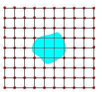
Suppose that somebody is standing at each red grid point with a watch. When the front crosses each grid point, the person standing there writes down this crossing time T. This grid of crossing time values T(x,y) determines a function; at each grid point T, T(x,y) gives the time at which the front crosses the point (x,y).

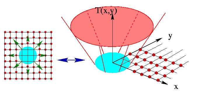
As an example, suppose the initial disturbance is a circle propagating outwards. The original region (the blue one on the left below) propagates outwards, crossing over each of the timing spots. The function T(x,y) gives a cone-shaped surface, which is shown on the right. This surface has a great property; it intersects the xy plane exactly where the curve is initially. Better yet, at any height T the surface gives the set of points reached at time T. The surface on the right below is called the arrival time surface, because it gives the arrival time.

Why is this called a "boundary value formulation"?

The reason it is called a "boundary value formulation" is because we have let the initial position of the front be the boundary for this arrival time surface T(x,y) that we would like to find. We have taken the idea of finding something that moves in time an exchanged it for a stationary problem in which the arrival surface contains the information about what is moving.

Why is this a good idea?

The reason this is a good idea is two-fold. First, even if the evolving front changes shape, the arrival time surface T(x,y) is nice and well-behaved. By slicing it with a saw at height T (that is, finding the level set T), it will always give the position of the front at time T.

The second reason to do this, as we will see below, is that there is an incredibly fast way to solve this, known as the Fast Marching Method.

The Fast Marching Method

How can this stationary surface be constructed? As a motivation, imagine scaffolding being erected around a house! One stands on one of the boards, puts a board above the head, and then moves to another board at the same level and put a board one level up. Once all the boards are placed at a given level, one then climbs up to the next level set repeat the process. The thing to remember is that the scaffolding is built from the ground up; each level must be completed before the next is begun.

The Fast Marching Method imitates this process. Given the initial curve (shown in red), stand on the lowest spot (which would be any point on the curve), and build a little bit of the surface that corresponds to the front moving with the speed F. Repeat the process over and over, always standing on the lowest spot of the scaffold, and building that little bit of the surface. When this process ends, the entire surface has been built.

(354K)

Construction of stationary level set solution

Green squares show next level to be built

The speed from this method comes from figuring out in what order to build the scaffolding; fortunately, there are lots of fast sorting algorithms that can do this job quickly.

Background and History: The Fast Marching Method, Dijkstra's Method, Tsitsiklis' Method, and Ordered Upwind Methods

The Fast Marching Method is very closely related to Dijkstra's method, which is a very well-known method from the 1950's for computing the shortest path on a network. Dijkstra's method is ubiquitous: everywhere from internet routing to your car's navigation system. To explain the connection, consider a network in which there is cost assigned to entering each node.


Find the shortest path from Start to Finish	Shortest path shown in Red

Dijkstra's method is an extraordinarily clever way to solve this problem. The basic idea is as follows:

Put the starting point in a set called "Accepted".
Call the grid points which are one link away from the Start "Neighbors".
Compute the cost of reaching each of these Neighbors.
The smallest of these Neighbors must have the correct cost. Remove it, and call it "Accepted." Add any new Neighbors to this point that are not already "Accepted", and find the cost of reaching all Neighbors. Repeat this step until there all points are Accepted.

This is an appealing algorithm. What it is doing is ordering the way in which the cost of reaching points are accepted, systematically working its way out from the known costs (the starting point) all the way to the finish. The method can be very made very fast: it is one-pass, because each point is touched essentially only once.

Solving the Continuous Eikonal Problem:

It is not too hard to see that this method cannot converge to the solution of a continuous Eikonal problem. No matter how much you refine the mesh, you will still get stairstep patterns: you can never find the diagonal that you want. This is where the Fast Marching Method comes in: it uses upwind difference operators to approximate the gradient, but retains the Dijkstra idea of a one-pass algorithm. It allows this methodology to be used to compute a large class of continuous problems.

Tsitsiklis (see the reference below) was the first to develop a Dijkstra-like method for solving the Eikonal equation: his was a control theory approach (as opposed to the Fast Marching upwind finite difference perspective) to solving the Eikonal equation: it is also a viscosity solution with the same operation count. This leads to a causality relationship based on the optimality criterion rather than on the upwind finite difference operators employed in Fast Marching Methods. In the particular special case of a first order upwind finite difference for the Fast Marching Method on a square mesh, the resulting update equation at each grid point can be seen to be the same quadratic equation obtained through Tsitsiklis's control theoretic approach. There are similarities and differences between his approach and Fast Marching Methods, we refer the interested reader to the paper on Ordered Upwind Methods (see the reference below) which discusses his approach in detail.

Finally, the advent of Ordered Upwind Methods allowed the Dijkstra-like methodology to be extended to a far wider class of problems, including continuous anisotropic static convex Hamilton-Jacobi equations, all with the same Dijkstra-like one pass flavor.

What is the difference between Fast Marching Methods and Level Set Methods?

Fast Marching Methods are designed for problems in which the speed function never changes sign, so that the front is always moving forward or backward. This allows us to convert the problem to a stationary formulation, because the front crosses each red grid point only once. This conversion to a stationary formulation, plus a whole bunch of numerical tricks, gives it its tremendous speed

Level Set Methods are designed for problems in which the speed function can be positive in some places are negative in others, so that the front can move forwards in some places and backwards in others. While significantly slower than Fast Marching Methods, embedding the problem in one higher dimension gives the method tremendous generality.

Details

Fast Marching Methods

The Fast Marching Method solves the general static Hamilton-Jacobi equation, which applies in the case of a convex, non-negative speed function. Starting with an initial position for the front, the method systematically marches the front outwards one grid point at a time, relying on entropy-satisfying schemes to produce the correct viscosity solution. The main idea is exploit a fast heapsort technique to systematically locate the proper grid point to update, so that one need never backtrack over previously evaluated grid points. The resulting technique sweeps through a grid of N total points in N log N steps to obtain the evolving time position of the front as it propagates through the grid. For details, see the technical explanations and flow chart.

References:

A Note on Two Problems in Connection with Graphs, : Dijkstra, E.W., Numerische Mathematic, 1:269--271, 1959.
Efficient Algorithms for Globally Optimal Trajectories : Tsitsiklis, J.N., IEEE Transactions on Automatic Control, Volume 40, pp. 1528-1538, 1995.
A Fast Marching Level Set Method for Monotonically Advancing Fronts : Sethian, J.A., Proc. Nat. Acad. Sci., 93, 4, pp.1591-1595, 1996. This paper List of downloadable publications
Ordered Upwind Methods for Static Hamilton-Jacobi Equations : Sethian, J.A., and Vladimirsky, A., Proceedings of the National Academy of Sciences, 98, 11069-11074, 2001. This paper List of downloadable publications
Ordered Upwind Methods for Static Hamilton-Jacobi Equations: Theory and Algorithms : Sethian, J.A., and Vladimirsky, A., SIAM J. Numer. Anal., 41, 1, pp. 325-363, 2003 This paper List of downloadable publications