HOME

OVERVIEW

APPLICATIONS

INTERACTIVE APPLETS

HISTORY OF THE METHODS/FLOW CHART

PUBLICATIONS

EDUCATIONAL MATERIAL

ABOUT THE AUTHOR/CV

Copyright:
1996, 1999, 2006
J.A. Sethian

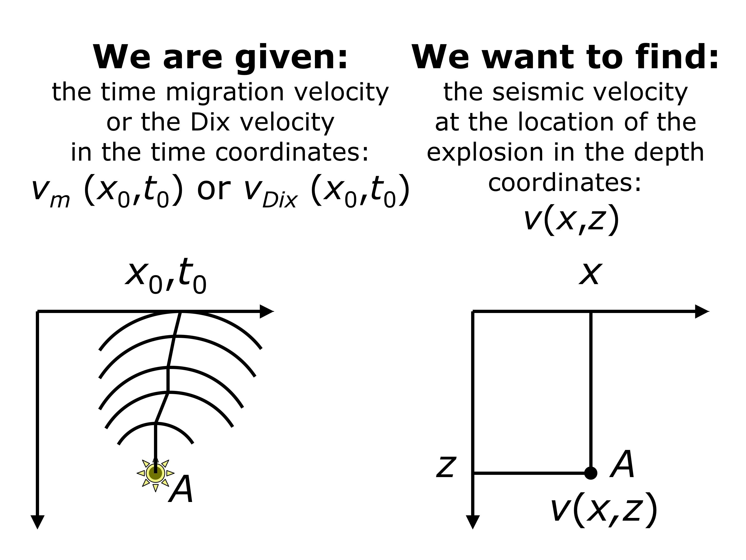
Seismic velocity estimation

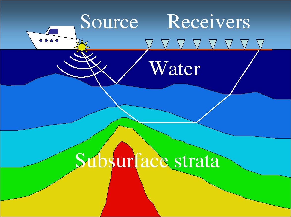
Imagine a boat producing explosions at equal intervals of time. The pressure waves propagate down to the seabed and deeper into the earth and reflect from all of the layer boundaries. Then the amplitudes of the reflected signals are recorded by receivers on the cable pulled by the boat. These records are the typical seismic data.

Our goal is to build a fast and robust algorithm for finding the sound speed inside the earth (so called "seismic velocity") from these data. Why is this important? Seismic velocity is necessary for obtaining accurate seismic images - images of layers and cracks inside the earth. These images are very helpful for determining, for example, where to drill for oil. Often oil gets trapped at the sides of a salt dome schematically shown here by the red color. Typically, salt is light and it pushes the layers up as it rises from inside the earth.

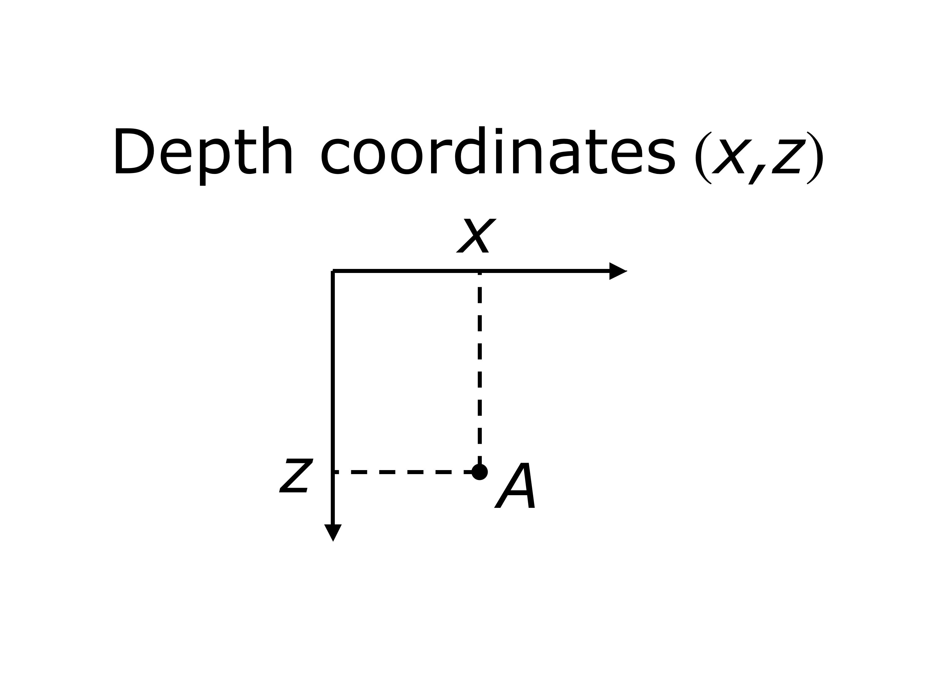
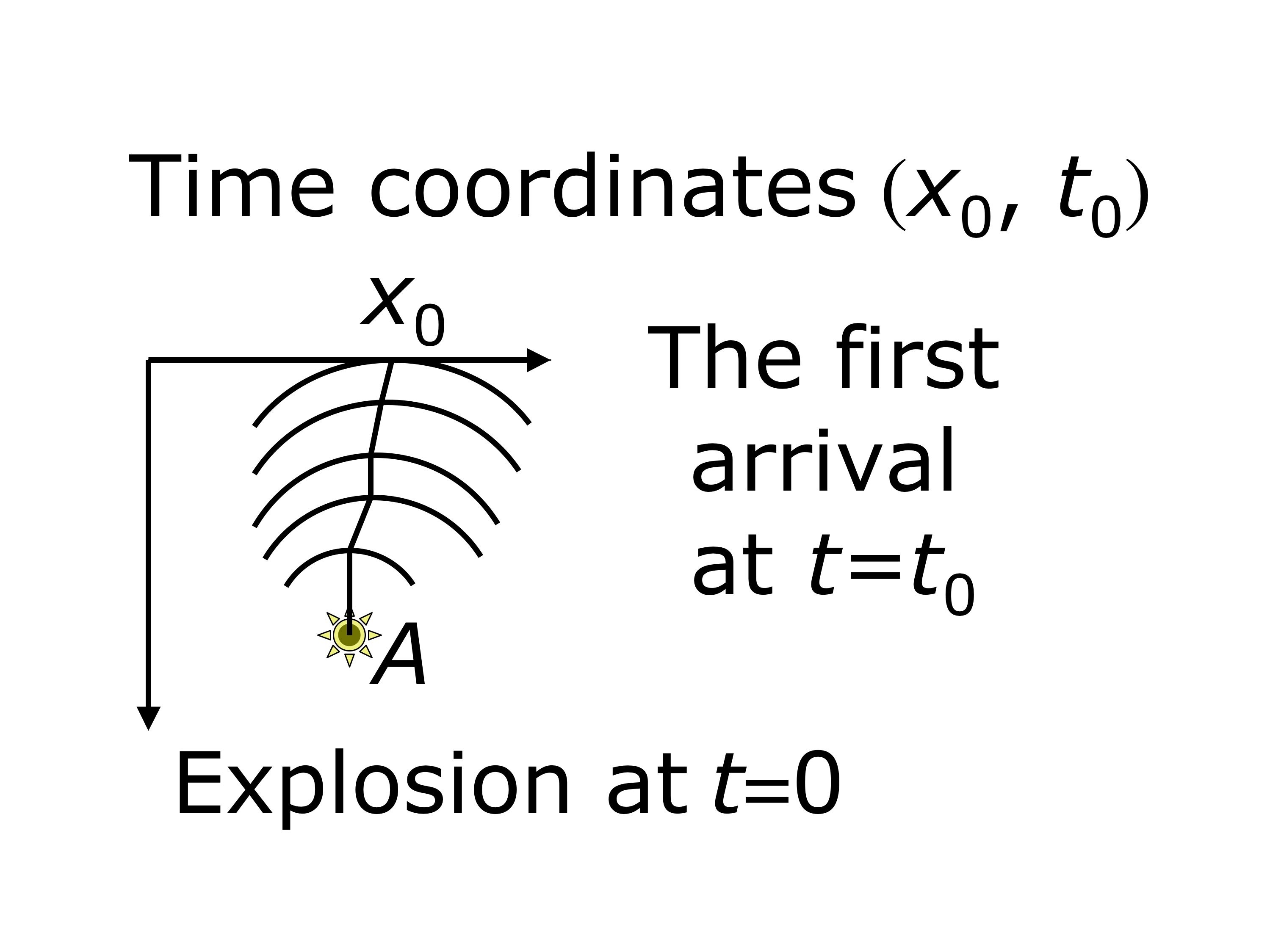
Time and depth coordinates
A location of a point A inside the earth can be described in the two following coordinate systems:

What are the problems with the existing seismic imaging?

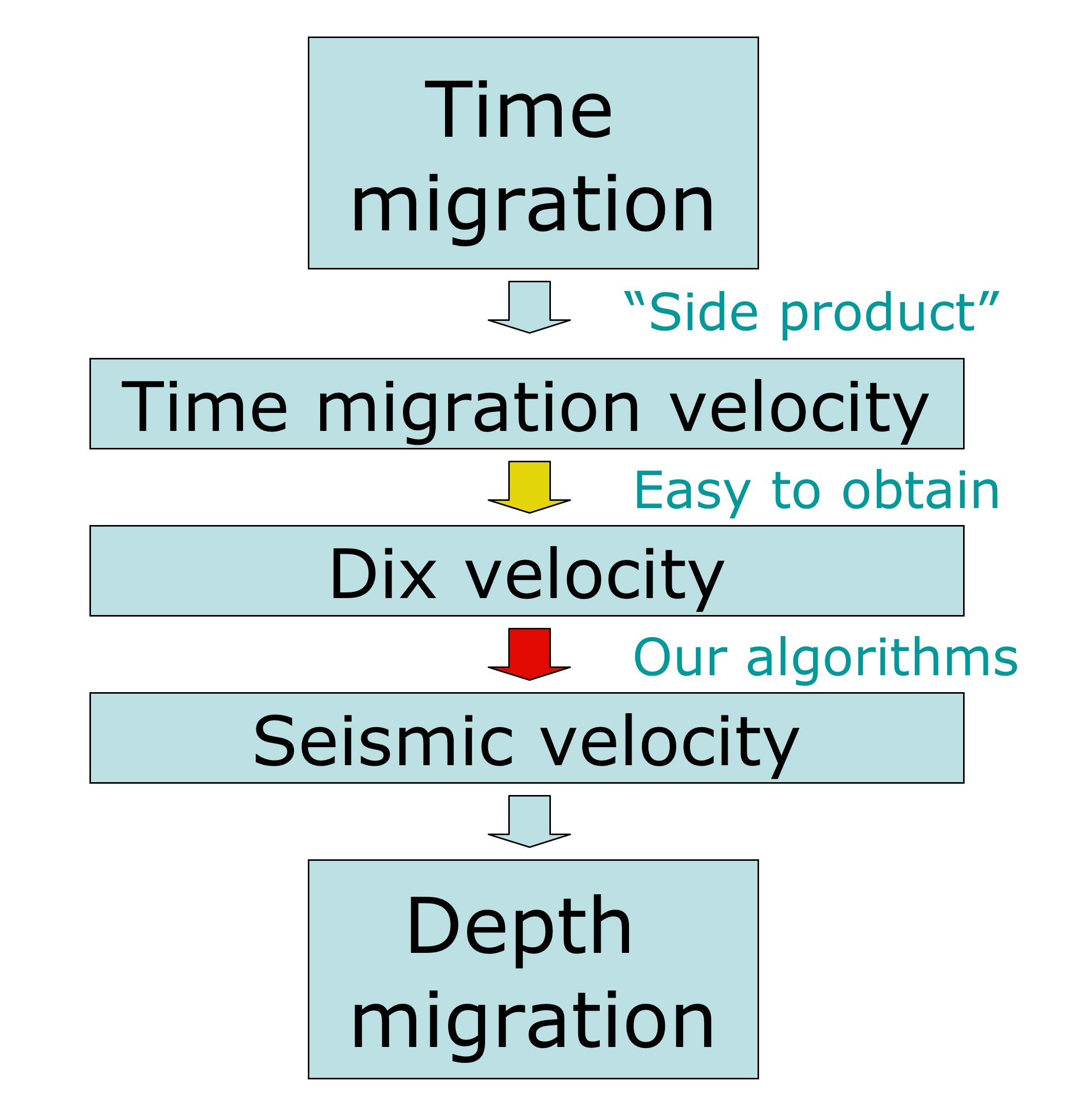
Nowadays there are two approaches to seismic imaging called time migration and depth migration. Time migration is fast and efficient but:

it is adequate for areas where the seismic velocity depends almost only on the depth, while oil tends to lie and all interesting phenomena tend to occur in the areas where the flat horizontal structures inside the earth are distorted;
it produces images in the time coordinates which relate to the regular Cartesian coordinates (the depth coordinates) in a very subtle way if the velocity depends on the lateral coordinates.
Depth migration produces images in the regular Cartesian coordinates and it is adequate for arbitrary areas. But one needs to know the seismic velocity to implement it. Naturally, the seismic velocity is never known. Typically, it is found by "guessing and trying".

Time migration Depth migration

Adequate for areas with mild lateral velocity variation arbitrary areas

Implementation requires nothing seismic velocity

Produces images in time coordinates depth coordinates

The central idea

Time migration produces so called time migration velocity as a "side product". This velocity is close to the root-mean-square velocity if the seismic velocity inside the earth depends only on the depth. If it is not so, it is some kind of mean velocity. The main idea of this work is

to understand how this time migration velocity relates to the true seismic velocity and
construct a numerical algorithm producing the seismic velocity from the time migration velocity.
Then this true seismic velocity can be used for the depth migration.
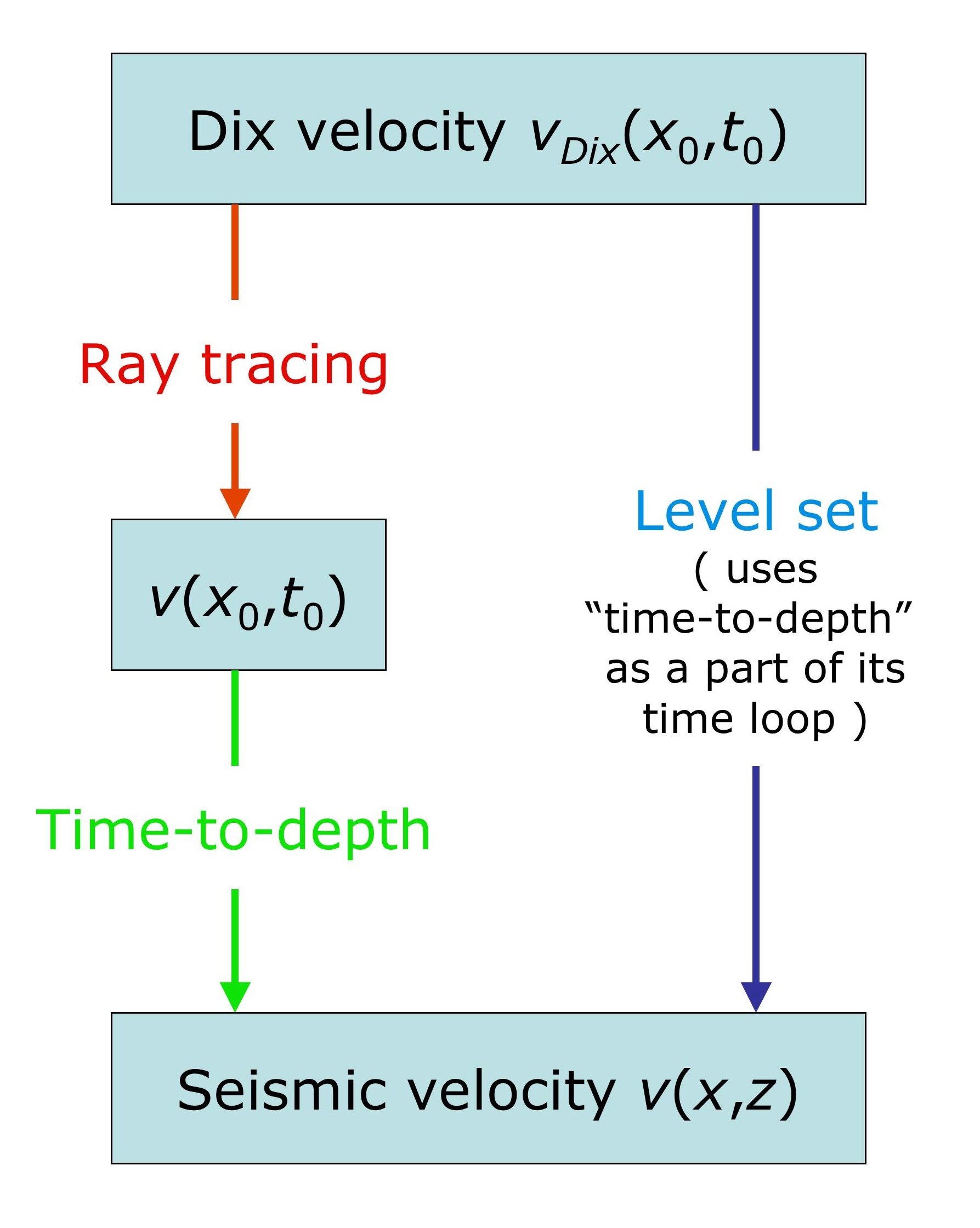
In 1955 an american geophysicist C. Hewitt Dix published a work on how the time migration velocity relate to the seismic velocity for the case of flat horizontal layers and velocity constant within each of them. Nowadays his method ("Dix conversion") is still in use. The result of application of his formula to the time migration velocity is called the Dix velocity. For convenience, we use the Dix velocity rather than the time migration velocity as the input for our numerical algorithms. The conventional method for finding the seismic velocity from the time migration velocity is the Dix method. It is adequate only for the flat horizontal layers and seismic velocity depending only on the depth. As we show in the present work, it may qualitatively differ from the true seismic velocity.

The inverse problem

The main results

Relation between the time migration velocity and the true seismic velocity in 2D and 3D.
Three numerical algorithms constructing the seismic velocity from the time migration velocity with some limitations:

an efficient time-to-depth conversion algorithm
an algorithm based on the ray tracing approach
an algorithm based on the level set approach

Numerical algorithms

The propagation of the pressure wave front can be described by the Eikonal equation. Its right-hand side is the unknown seismic velocity.

Time-to-depth conversion algorithm solves the Eikonal equation with an unknown right-hand side together with an orthogonality relation. Its motivation and a building block was the fast marching method . Due to the fact that the RHS of the Eikonal equation is unknown, a very subtle issue appears and makes this extension nontrivial. This algorithm is used in the other two algorithms as their essential part. Used by itself, it produces results of the same quality as the conventional methods in seismic imaging, but its advantage is its speed and robustness.
Ray tracing algorithm first solves a system of ray (characteristic) equations for the Eikonal equation as well as the equations for the quantities involved into the relation between the time migration velocity and the seismic velocity. Then the time-to-depth conversion algorithm is used as its final step. This approach is fast, however it fails when the rays start to come too close to each other or spread too strongly.
Level set algorithm is based on the level set methods . It uses the time-to-depth conversion algorithm as a part of its time loop. This algorithm is slow in comparison with the ray tracing algorithm, but it does not necessarily fail when the rays cross: it follows the "first arrival front".
We showed on the synthetic data examples that the last two algorithms can significantly improve the accuracy of the found seismic velocity while the conventional approach based on the Dix method can produce qualitatively wrong results.

The main difficulty and its resolution
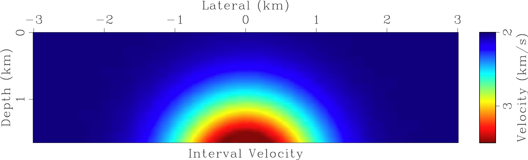
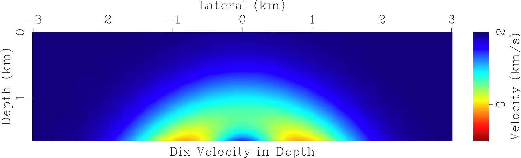
We showed that the problem of constructing the seismic velocity from the Dix velocity is very ill-posed. We used the least square polynomial approximation to suppress the tiny but sharp "bumps" in the seismic velocity under construction.
Synthetic data example
The exact velocity The input data: the Dix velocity The found velocity and the rays
Field data example

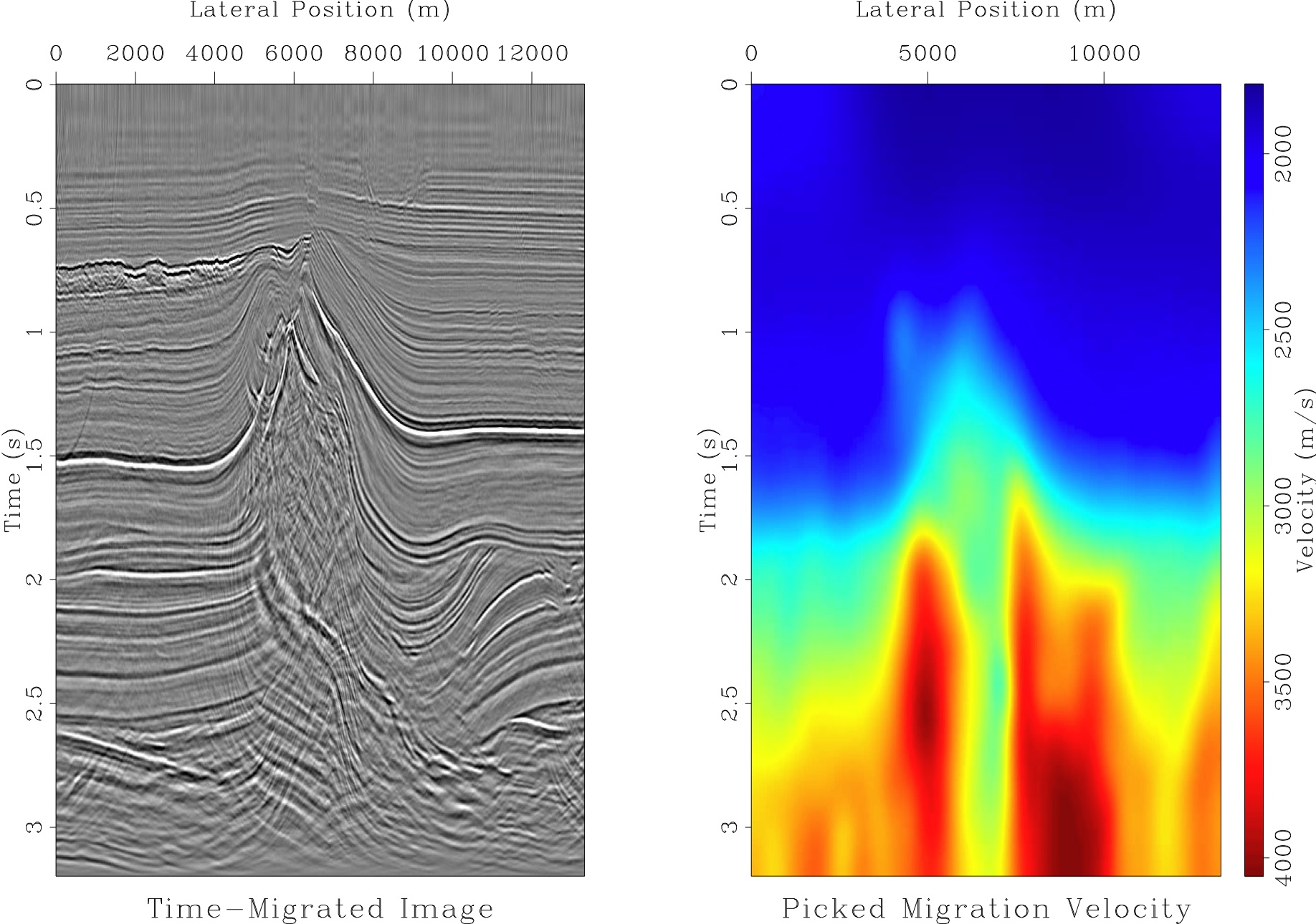
Left: seismic image from the North Sea obtained by the time migration. Right: the corresponding time migration velocity.

The image is in the time coordinates. The main feature in it is the salt dome in the middle. typically, the seismic velocity of the salt is high in comparison with it of the surrounding rock. Note a mess inside the salt dome which indicates that the lateral velocity variation is too severe for the time migration.

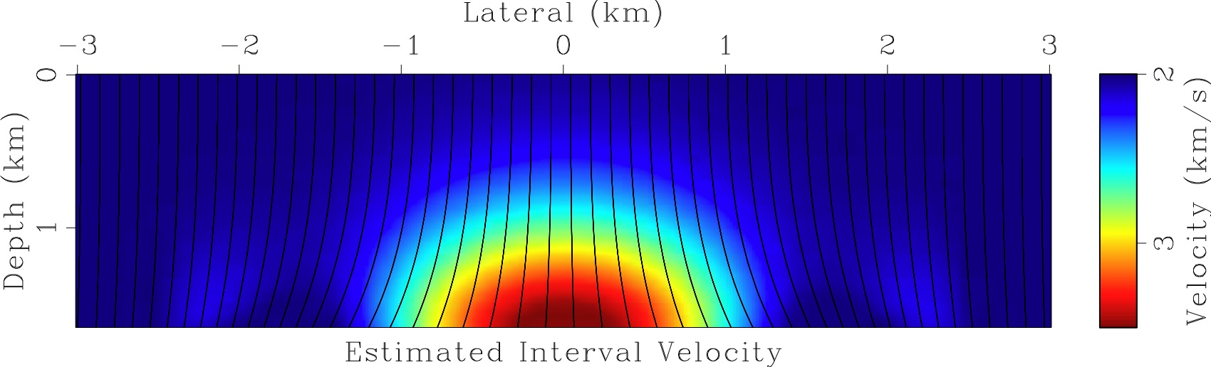
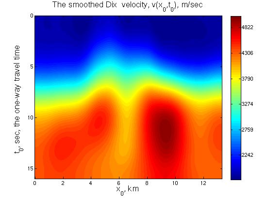
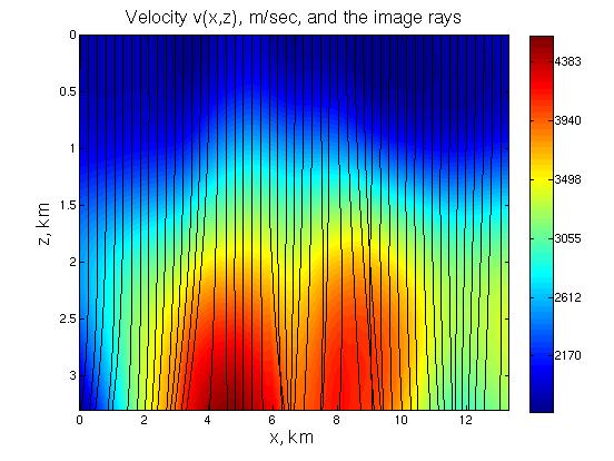
Left: the input data: the Dix velocity.
The Dix velocity was obtained from the time migration velocity shown in the figure above and then smoothed.

Right: the seismic velocity found by our level set algorithm, and the image rays computed for the found velocity. Note that they diverge and intersect and our algorithm successfully handled this. The seismic velocity was cut off at 3.3 km in depth to make the velocity array rectangular.

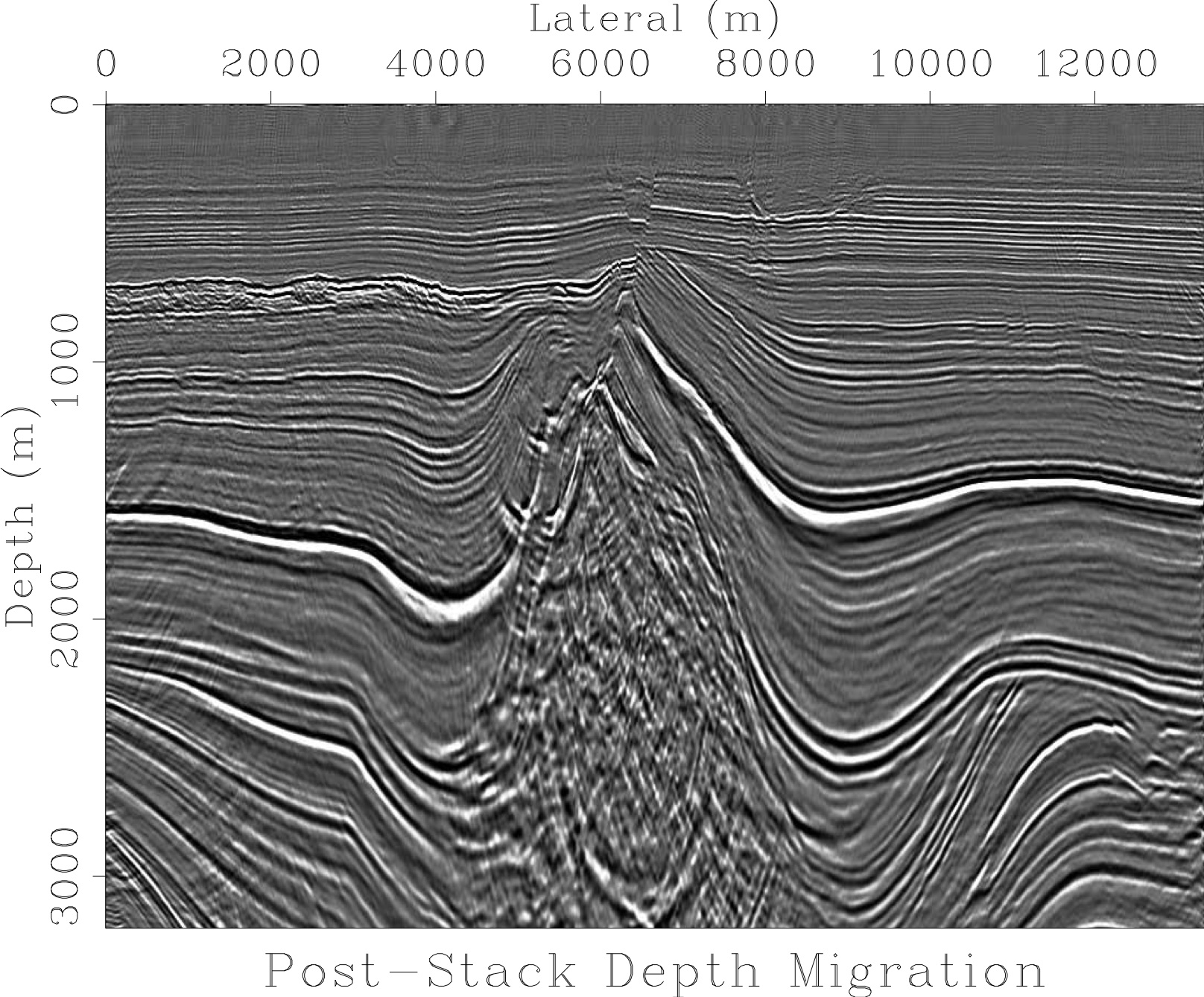
The depth migrated image of produced using the seismic velocity found by our level set algorithm.
The image is in the depth (regular Cartesian) coordinates. It is up to 3.3 km in depth which is quite deep according to the geophysical standards. There is a mess inside the salt dome but the surrounding layers are resolved well. Overall, this image looks reasonable.

References

Seismic Velocity Estimation using Time Migration Velocities ,
Cameron, M. K., Fomel, S. B., Sethian, J. A., J. Comp. Phys., 2006, in progress.