HOME

OVERVIEW

APPLICATIONS

INTERACTIVE APPLETS

HISTORY OF THE METHODS/FLOW CHART

PUBLICATIONS

EDUCATIONAL MATERIAL

ABOUT THE AUTHOR/CV

Copyright:
1996, 1999, 2006
J.A. Sethian

Seismic velocity estimation

The goal of this work is to build a fast and robust algorithm for finding the sound speed inside the earth (so called "seismic velocity") using only data measured on the surface: pressure wave amplitudes as functions of the locations of sources and receivers and the travel times between them.

Why is this important?

Seismic velocity is necessary for obtaining accurate seismic images - images of layer boundaries and cracks inside the earth. These images are very important for determination where to drill for oil, for investigation of the earthquakes, etc. ... In the present work we use the terminology from the oil industry.

What are the problems with the existing seismic imaging?

Nowadays there are two approaches to seismic imaging called time migration and depth migration. Time migration is a fast and efficient procedure routinely applied to the seismic data. The problems with it are:

it is adequate for areas with mild lateral velocity variation, while oil tends to lie and all interesting phenomena tend to occur in the areas where the flat horizontal structures inside the earth are distorted;
it produces images in very specific so called time migration coordinates which relate to the regular Cartesian coordinates in the case of the lateral velocity variation in a very subtle way.
Depth migration produces images in the regular Cartesian coordinates. It is adequate for arbitrary areas, but its implementation requires the knowledge of the seismic velocity. An iterative approach of guesswork followed by correction is often employed. The time migration coordinates

The central idea
Time migration produces some kind of mean velocities so called time migration velocity as a "side product". The main idea is

to understand how this time migration velocity relates to the true seismic velocity and
construct a numerical algorithm producing the seismic velocity from the time migration velocity.
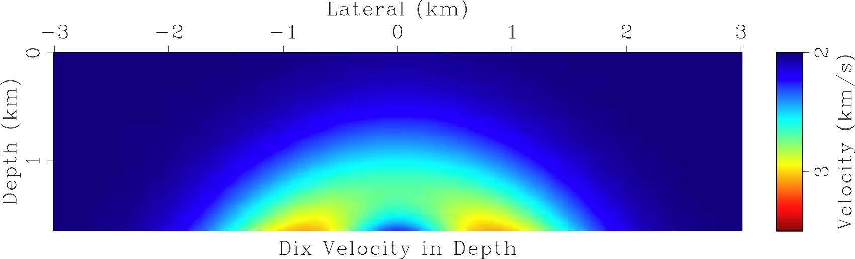
Then this true seismic velocity can be used for the depth migration.
The conventional method for finding the seismic velocity from the time migration velocity is the Dix method. It is adequate only for the flat horizontal layers and seismic velocity depending only on the depth. As we show in the present work, it may qualitatively differ from the true seismic velocity.

Dix conversion is a fast, simple and routine procedure. For convenience, we take the Dix velocity - the result of the Dix conversion as the input data for our algorithms.

The main results

Relation between the time migration velocity and the true seismic velocity in 2D and 3D.
Three numerical algorithms constructing the seismic velocity from the time migration velocity with some limitations:

an efficient time-to-depth conversion algorithm
an algorithm based on the ray tracing approach
an algorithm based on the level set approach

Numerical algorithms
The propagation of the pressure wave front can be described by the Eikonal equation. Its right-hand side is the unknown seismic velocity.

Time-to-depth conversion algorithm solves the Eikonal equation with an unknown right-hand side together with an orthogonality relation. Its motivation and a building block was the fast marching method . Due to the fact that the RHS of the Eikonal equation is unknown, a very subtle issue appears and makes this extension nontrivial. This algorithm is used in the other two algorithms as their essential part. Used by itself, it produces results of the same quality as the conventional methods in seismic imaging, but its advantage is its speed and robustness.
Ray tracing algorithm first solves a system of ray (characteristic) equations for the Eikonal equation as well as the equations for the quantities involved into the relation between the time migration velocity and the seismic velocity. Then the time-to-depth conversion algorithm is used as its final step. This approach is fast, however it fails when the rays start to come too close to each other or spread too strongly.
Level set algorithm is based on the level set methods . It uses the time-to-depth conversion algorithm as a part of its time loop. This algorithm is slow in comparison with the ray tracing algorithm, but it does not necessarily fail when the rays cross: it follows the "first arrival front".
We showed on the synthetic data examples that the last two algorithms can significantly improve the accuracy of the found seismic velocity while the conventional approach based on the Dix method can produce qualitatively wrong results.
The main difficulty and its resolution
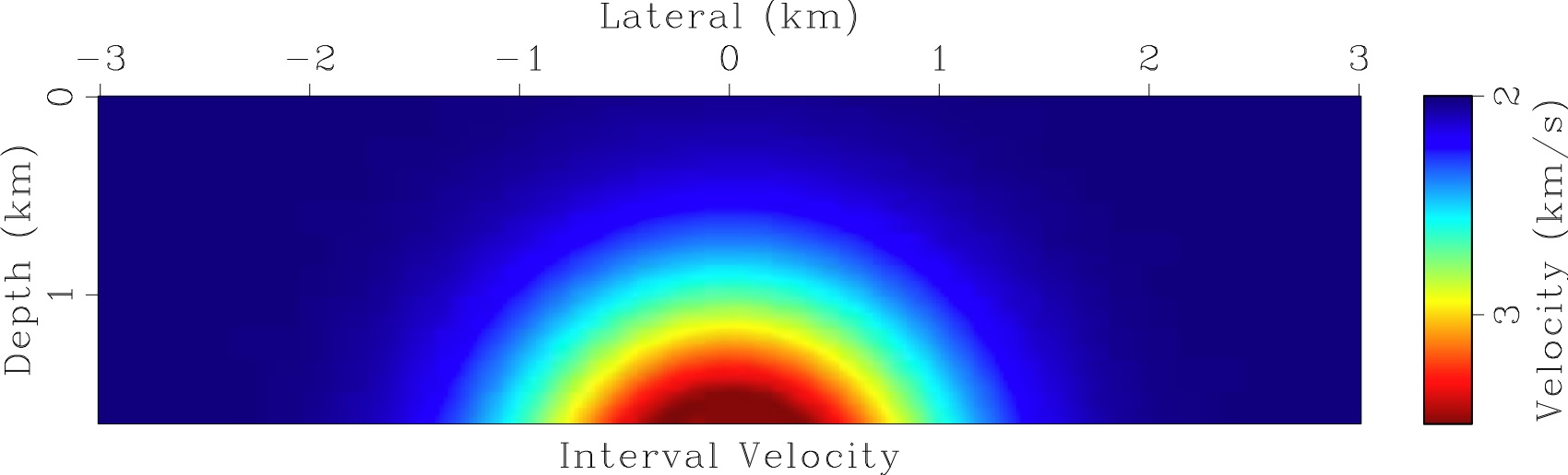
We showed that the problem of constructing the seismic velocity from the Dix velocity is very ill-posed. We used the least square polynomial approximation to suppress the tiny but sharp "bumps" in the seismic velocity under construction.
Synthetic data example
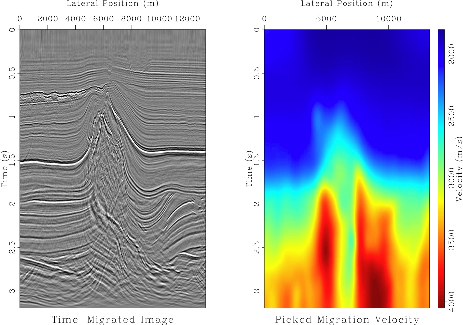
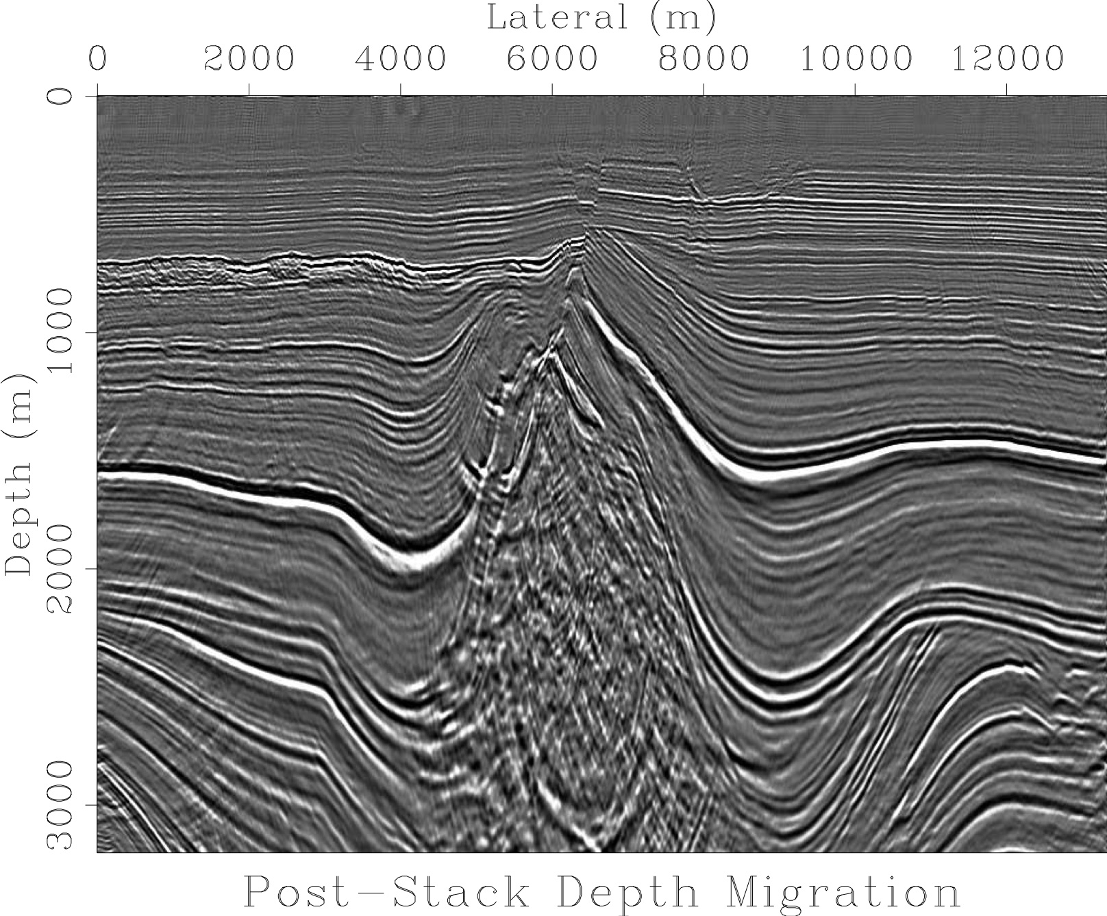
The exact velocity The input data: the Dix velocity The found velocity and the rays
Field data example

Left: seismic image from the North Sea obtained by the time migration. Right: the corresponding time migration velocity.

The input data: the Dix velocity.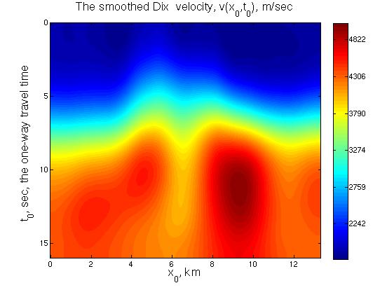
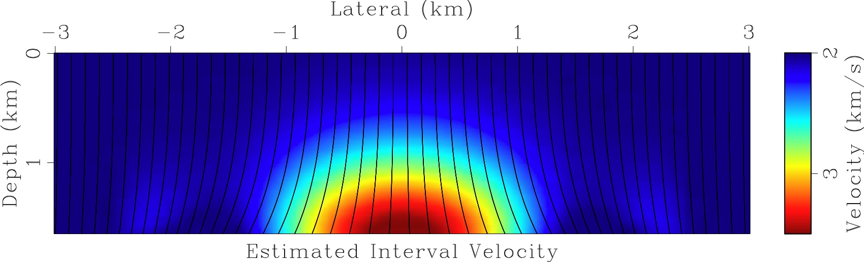
The found velocity and the rays.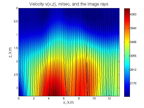

The depth migrated image obtained using the found seismic velocity References

Seismic Velocity Estimation using Time Migration Velocities ,
Cameron, M. K., Fomel, S. B., Sethian, J. A., J. Comp. Phys., 2006, in progress.