What are Gauss and Dowker-Thistlethwaite codes?

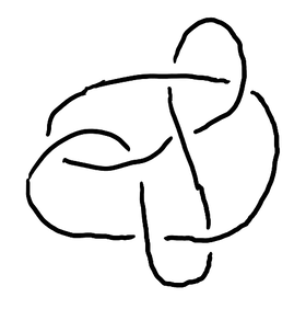
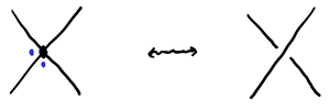
A popular way to study knots is to work with diagrams, which, formally speaking, are immersions of a circle in the plane along with the information about which of the two strands goes over the other at each crossing. The usual convention is to draw the under-strand with a gap, giving a sort of chiaroscuro effect that suggests the under-strand is just a little too far away to be lit. For example, here is how one might draw the knot $7_6$:

This represents something like the following knot tied into a loop of rope: Diagrams reduce the infinite complexity of all the ways a loop might be embedded in three-dimensional space to a finite amount of data. In this article, we will talk about exactly what this data is and some ways to represent it. The aim is to show how even a computer can do things with knots.

We will begin with how knot (and link) diagrams are planar graphs with additional crossing information, then discuss how to represent particular planar embeddings of a graph with combinatorial maps. From there, we will talk specifically about representing knots with Gauss codes, and then move to the more-efficient representation, Dowker-Thistlethwaite (DT) codes. It should be known that this comes at the cost of being unable to distinguish between mirror images of the same knot, and there is even more ambiguity for non-prime diagrams, though we’ll see a variation without this limitation.

The description of DT codes here — motivated through combinatorial maps — is done in a way I personally find to be less confusing, and hopefully you, who might have found this page in a search to understand them, will appreciate it.

1. Link diagrams as planar graphs

Recall that links are a generalization of knots: rather than having a single closed loop, a link is made of any number of closed loops embedded in three-dimensional space. There’s no harm in generalizing to this case, and it doesn’t really add any additional complexity (though we will go back to just considering knots when we get to Gauss codes and Dowker-Thistlethwaite codes). Links might be oriented, which pictorially is represented by an arrowhead somewhere along each link component.

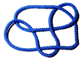
As you can find in most textbooks on knot theory, every link has a diagram. One way to get a diagram is to perturb the link slightly with an isotopy in a “generic” way and then project it down to a plane. Since isotopic knots and links are considered to be equivalent, one simplification we will make is to assume that, when there is a split diagram, no diagram component is “inside” any other by isotoping each component away from each other:

Diagrams themselves can be isotoped around, and any two isotopic diagrams are considered to be equivalent. With this in mind, what is the data of a diagram? In other words, if someone found a cool knot and wanted to tell someone about it, but they had to do it over the phone, what could they say to guarantee they are perfectly understood?

Something to notice about a diagram is that (1) it has crossings, which can be thought of as two short pieces of string overlapping at a single point, and (2) it has edges, which are the pieces of string that are between two crossings. This reductive kind of thinking gives us a $4$-regular planar graph, where the crossings become vertices.

The graph itself is certainly not enough to recover the knot, since it forgets which edges form the overstrand at each crossing. If we adapt Alexander’s notation^[1], we can use two blue dots to indicate how to interpret a vertex as a crossing:

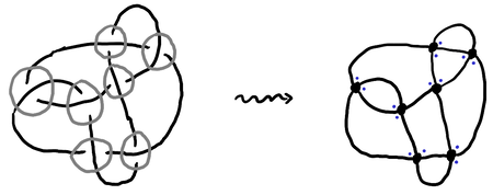
For this notation to make sense, the way in which the graph is embedded in the plane is important (at least up to isotopy). An answer to representing embeddings is called a combinatorial map. Let’s get a formal definition out of the way and not speak much of it again. A combinatorial map is a set $D$ of darts, an involution $\alpha$ of $D$ with no fixed points, and a permutation $\sigma$ of $D$. The orbits of $\alpha$ are the edges, and the orbits of $\sigma$ are the vertices.

What problem is this solving? We would like to have a way to know the cyclic order of incident edges around each vertex and how they are attached. As it turns out, if you know this, you can perfectly reconstruct the embedding of the planar graph^[2]. We would also eventually like to be able to deal with oriented links, which involves giving each edge of the graph an orientation, but if we just kept track of the order of edges around each vertex there is an issue when it comes to self loops: which end of the edge is attached in which order?

So what is a dart? I like to think about a dart as being half an edge, but you can also think of it as being a vector at an endpoint of an edge that points into the edge. Then, every edge has two darts, and for each vertex you record the cyclic order of the incident darts (say, going around counter-clockwise). All of this together is enough to reconstruct the planar embedding.

For link diagrams, you still need to know which darts participate in the overstrand and which participate in the understrand. One way to deal with this is to record the four darts in order as a list, but to make sure the first one in the list is for an understrand. That way, the first and third form the understrand, and the second and fourth form the overstrand. Cyclically shifting the darts over by two doesn’t change the meaning of the data.

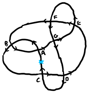
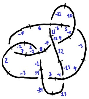
What we can do is take each edge of the diagram, subdivide it into two darts, then label them all with a number. It is convenient to make it so darts $2k+1$ and $2k+2$ correspond to the same edge — that way we don’t need to record the correspondence. For example, if we label the darts of $7_6$ like so:

then we can record the the combinatorial map in a table:

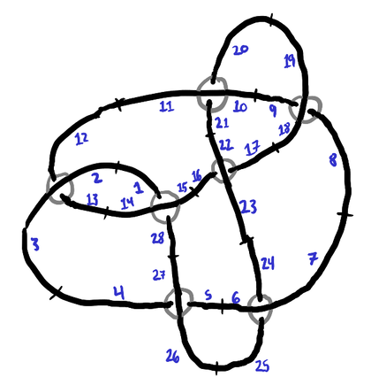
1	13	4	24	8	21	16
14	2	26	6	19	10	23
28	12	5	25	9	20	17
15	3	27	7	18	11	22

Each column corresponds to a different crossing (the order of the crossings does not matter), with the darts coming in counter-clockwise order around the crossing, and the first dart is one of the two darts corresponding to the understrand.

This is all there is to communicating a knot to someone, and everything else is merely an optimization. $4n$ numbers can be a lot to store, though (especially if you are someone like Ben Burton, who likes tabulating all knots up to some large number of crossings).

Before optimizing anything, it’s worth discussing things you can do with a diagram given in this representation:

• A dart with label $2k+i$, where $i\in \{0,1\}$, represents sitting at a crossing and facing in the direction of the dart. You can travel down the dart’s edge and sit at the other crossing, then about-face, just by calculating $\alpha (2k+i)=2k+1-i$.
• Given a dart $d$, one can rotate 90 degrees counter-clockwise and get a new dart $\sigma \left(d\right)$ by taking the next dart (cyclicly) in the list associated with the vertex for $d$.
• A dart represents an orientation of a link component. Walking along a link is repeatedly calculating $\sigma \left(\sigma \right(\alpha \left(d\right)\left)\right)$ to (1) flip across an edge then (2) rotate 180 degrees.
• You can represent an oriented link diagram by making edges be oriented in the $2k+1\to 2k+2$ direction, with respect to dart labels. This was done in the example above.
• Seifert circuits for oriented link diagrams are from taking an odd-labeled dart $d=2k+1$, then continuing along $\sigma \left(\alpha \right(d\left)\right)$ or ${\sigma }^{-1}\left(\alpha \right(d\left)\right)$, depending on which of the two is odd.
• Faces (which are useful for the Dehn presentation of the fundamental group of a link complement) come from the orbits of ${\sigma }^{-1}\circ \alpha$, at least for non-split diagrams. In a split diagram, we arranged for one of the faces to be a punctured disk, and for this face orbits instead give its boundary components.

When doing calculations on a computer, it seems to be a good idea to convert things into this representation first. At least, I’ve found it to be very convenient.^[3]

An optimization for diagrams with no self loops. If the diagram has no self loops (that is, it has no applicable Reidemeister I moves), then instead of labeling darts, you can get away with labeling edges, giving the small savings that each label needs one fewer binary digit that before (there being half as many labels). The orientation of a component can be recorded by labeling edges using consecutive numbers like so:

As before, the combinatorial data can be recorded in a table:

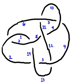
1	7	2	12	4	11	8
7	1	13	3	10	5	12
14	6	3	13	5	10	9
8	2	14	4	9	6	11

This is exactly the data of a Planar Diagram (PD) as used by KnotTheory and SnapPy. In the format of KnotTheory, this can be written as

PD[X[1,7,14,8], X[7,1,6,2], X[2,13,3,14], X[12,3,13,4],
   X[4,10,5,9], X[11,5,10,6], X[8,12,9,11]]

and in SnapPy, this can be written as

Link([(1,7,14,8), (7,1,6,2), (2,13,3,14), (12,3,13,4),
      (4,10,5,9), (11,5,10,6), (8,12,9,11)])

Unlike for the full combinatorial map, it is less convenient walking along various features of the diagram when it is in this format.

Remark. I have considered using a variant of PDs for oriented diagrams that uses the dart convention, so for example the first entry would be X[1,14,28,15] instead of X[1,7,14,8]. Parity gives orientations. Or, one could use positive and negative numbers to indicate dart orientations.

Unknots and paths. One thing I have swept under the rug is that the $0$-crossing diagram of an unknot has no crossings, so it cannot be represented in this way! We can fix this by allowing edges to be subdivided using degree-$2$ vertices. Then, in addition to a crossing table, we would have a paths table containing pairs of darts that are joined by the degree-$2$ vertices. In KnotTheory notation, the additional paths are represented using P inside the PD, so the $0$-crossing unknot would be

PD[P[1, 1]]

This extension makes it easy to implement the Kauffman bracket in Mathematica, as explained at The Kauffman bracket polynomial (see also The Knot Atlas).

Oriented crossings. Rather than orienting the edges, a variation that KnotTheory can use is an orientation at the crossings themselves in terms of the sign of the crossing. Each X is instead an Xp or Xm depending on whether the crossing is respectively positive or negative, given the following order for edge labels:

The knot $7_6$, oriented according to the edge labels from before, can be represented this way as

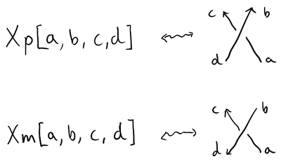
PD[Xp[14,8,1,7], Xp[6,2,7,1], Xm[2,13,3,14], Xm[12,3,13,4],
   Xp[4,10,5,9], Xp[10,6,11,5], Xp[8,12,9,11]]

2. Gauss codes

An early problem in “geometria situs” (now called combinatorial topology) considered by Gauss^[4], is the following. Given a generic oriented immersed loop in the plane (that is, an oriented closed loop that is allowed to self intersect only transversely and without triple points), one can label the double points and, beginning from some base point on the curve, read off these labels to form a word where every label appears exactly twice. The problem is the converse: under what circumstances does such a word correspond to some such planar curve?

Gauss presumably considered this problem because these curves are the shadow of a knot, and it is a reasonable first step to study what knots exist — later one might introduce crossings.

Remark. While Gauss called these generic immersed loops knoten, they are certainly not knots.

There is a lot to say about the Gauss word realization problem (which Gauss did not fully solve!), but it would take us too far afield. I refer you to Jeff Erickson’s nice notes on planar curves from his course One-dimensional computational topology.^[5]

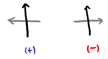
Closer to what we need is the idea of a signed Gauss word. Rather than just writing down the labels, we also record the orientation of the other strand through the double point, which is done using the sign of the determinant of the tangent vectors of both strands at the double point (that is, the signed intersection number). In the following, the gray strand is the other strand.

For example, with the shadow of $7_6$, the oriented code from the turquoise basepoint is $$\overline{A}BC\overline{D}\overline{E}F\overline{B}A\overline{G}E\overline{F}GD\overline{C},$$ where $\overline{L}$ means $L$ with negative sign. Notice each label appears with both signs.

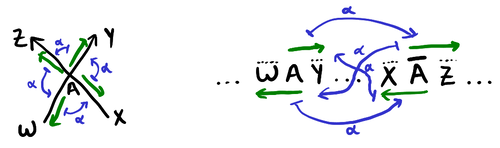
A signed Gauss word should be thought of as being a compact representation of a combinatorial map that is an oriented knot shadow (characterized by having every vertex be degree $4$ and having exactly one oriented circuit). For example, consider the edge $\overline{A}B$. We can give $\overline{A}B$ and $B\overline{A}$ as labels for its two darts, and all these names will be unique across all darts. Then, the cyclic order of the darts incident to a vertex comes from directly from a Gauss word as illustrated in the following diagram, where the green arrows represent the darts:

This is meant to represent that the following is the counter-clockwise cyclic order of the darts incident to $A$, given that the signed Gauss word contains $W^{\pm }A{Y}^{\pm }$ and $X^{\pm }\overline{A}{Z}^{\pm }$: $$A{Y}^{\pm }\mapsto \overline{A}{Z}^{\pm }\mapsto A{W}^{\pm }\mapsto \overline{A}{X}^{\pm }\mapsto A{Y}^{\pm }.$$

The following theorem shows the degree to which signs are needed for reconstructing knot shadows.

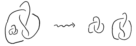
A knot shadow is called prime if, as a $4$-regular graph, it is $3$-edge-connected. An equivalent definition is that, for every circle that transversely intersects the shadow in exactly two points away from the double points, at least one side of the circle has no double points. Yet another equivalent definition is that no cyclic permutation of its Gauss word is the concatenation of two Gauss words. Prime knots have prime knot shadows.

Theorem. If two prime knot shadows have the same unsigned Gauss word (allowing relabeling and change of basepoint), then either they are isotopic (in $S^2$) or are mirror images.

Proof. The choice of signs in a Gauss word is a choice for each vertex of whether the above cyclic order is clockwise or counter-clockwise. Consider two knot shadows $S_1$ and $S_2$ (on $S^2$) with equivalent unsigned Gauss words. Color $S^2$ white, and for each double point of $S_2$ that has reversed orientation from the corresponding double point of $S_1$, place a black disk on the double point. Now, wherever there are adjacent double points with black disks, join the black disks together along the edge. This might give monochromatic white disks that do not contain any of $S_2$ — color these black. The result is a collection of black regions that can be thought of as being regions of $S_2$ with reversed orientations from $S_1$. If there is both a black and a white region, there is a black or white disk region — assume it is black. Its boundary is a circle that avoids double points and intersects $S_2$ transversely, so by primality (and the Jordan curve theorem) it must intersect $S_2$ at least four times. But this is a contradiction, because flipping the portion of $S_2$ inside the disk over would enlarge the portion of the graph that matches the orientation of $S_1$, but flipping this portion results in a non-planar graph. Therefore there is exactly one region, implying $S_2$ is either isotopic to $S_1$ or a mirror image of it. QED

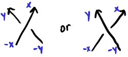
Now what about knots? Since we now understand the correspondence between a signed Gauss word and its combinatorial map, we know all we need to indicate is the over and under information so the double points become actual crossings, and this will give the (signed) Gauss code of the knot.

One thing you should avoid being confused about if you can help it: the right-handed and left-handed crossings are also known as positive and negative crossings, respectively. This use of positive and negative is distinct from their use in Gauss words. For crossings, it is contribution to linking number, but for double points it is the signed intersection number.

We can indicate the crossing types by recording along with the sign of the intersection whether the strand goes over or under. So, for $7_6$ with crossings labeled like so

we can write down the signed Gauss code $$\overline{A^U}{B}^O{C}^U\overline{D^O}\overline{E^U}{F}^O\overline{B^U}{A}^O\overline{G^U}{E}^O\overline{F^U}{G}^O{D}^U\overline{C^O}.$$ The fact the diagram is an alternating diagram is reflected in the alternating $U$’s and $O$’s.

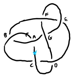
Using the theorem from the previous section, if we only care about a prime knot up to mirror image, we can omit the intersection signs. It is common then to have $-A$ denote $A^U$ and $A$ denote $A^O$, so the above code becomes an unsigned Gauss code

$$-A,B,-C,D,-E,F,-B,A,-G,E,-F,G,-D,C.$$ (The actual notations used for Gauss codes can vary, but what is universal is the idea of recording visited vertices, over and under information, and possibly intersection signs for the shadow.)

As a matter of normalization, we can “multiply” this by $-1$ so that the first letter is always positive, since the unsigned Gauss code only determines the knot up to mirror image anyway. Another thing we can do is consider all cyclic shifts and relabelings and take the lexicographically minimal one. Using numeric indices instead of letters, according to KnotInfo the lexicographically minimal Gauss code (also allowing orientation reversal) is

$$1,-2,3,-4,5,-6,7,-3,2,-7,6,-1,4,-5.$$

A quick space usage analysis. In an $n$-crossing knot diagram, a Gauss code will have $2n$ terms each adorned with $O$ or $U$ and possibly an intersection sign. For over and under information, we only need to record whether it is the first or second instance of the label that is over, and intersection sign is similar. Since we can normalize the labeling so that the letters are introduced in order, the number of unsigned Gauss words with $n$ labels is counted by $\frac{\left(2n\right)!}{n!2^n}$ (planar or not). Putting this together, there are $2^n\frac{\left(2n\right)!}{n!}$ signed Gauss words. The logarithm base $2$ of this gives a theoretical lower bound on the number of bits required to encode one, and there is an approximation

$${\log }_2\left(2^n\frac{\left(2n\right)!}{n!}\right)\approx n{\log }_{2}n+(3-\ln (2{)}^{-1})n+\frac{1}{2},$$ where their difference tends to $0$ for large $n$. Thus, the number of bits to store a signed Gauss code has the following rough upper bound (good to a few decimal places): $$n{\log }_{2}n+1.557n+\mathrm{0.5.}$$ Subtract $n$ to get the bits for an unsigned Gauss code. This does not take into account the fact we need to store $n$ itself (using roughly ${\log }_{2}n$ bits). One approach is to fix some $n$ for all knots under consideration and use obvious Reidemeister I moves to pad the representation. Another is to have one table per $n$.

The following table shows how large of a knot diagram can be stored in a given number of bytes, where the representation is either a signed Gauss code or an unsigned Gauss code.

Bytes	Signed Gauss code max crossings	Unsigned Gauss code max crossings
8	12	14
16	21	24
32	37	42
64	67	75

3. Dowker-Thistlethwaite codes

Dowker and Thistlethwaite modified Tait’s original notation for the purpose of tabulating knots by computer. First let’s quickly see their definition, and then we will relate this to combinatorial maps. For the double points in a knot shadow, consider the preimages, which we may number consecutively by $1,2,\dots ,2n$, and thus the pairs of numbers assigned to a double point defines an involution $a$ on the set $\{1,2,\dots ,2n\}$. They use the fact that this involution sends even numbers to odd numbers, and vice versa, so the sequence $\left(a\right(1),a(3),\dots ,a(2n-1\left)\right)$ determines the involution. They then use negative signs to record the crossing type, where $a(2k+1)$ gets a negative sign if the point $2k+1$ of the knot corresponds to the overstrand.^[6][7]

A different way of assigning labels to darts in an oriented knot shadow is to (1) assign $1,2,3,\dots$ to edges in consecutive order along the knot’s orientation, (2) for each dart that points in the direction of the orientation, label it with its edge label, and (3) for each dart that points in the opposite direction, label it with the negative of the label opposite it at the crossing. That is, (a) the sign of each dart corresponds to whether or not it is co-oriented with the knot, (b) the absolute values of the darts are non-decreasing with respect to the orientation of the knot, (c) along each edge the darts are labeled $x\to -x-1$, and (d) around each crossing the darts satisfy the following labelings:

For example, labeling $7_6$ gives

Looking at the labels around a crossing, there seems to be a lot of redundancy, like somehow only two of the four numbers might be needed.

For the same reason that the involution described by Dowker and Thistlethwaite is parity reversing, every crossing has darts that are even and odd. One way to see this is that if you took an arc of a knot whose projection is a path from a crossing to itself, then the $Z/2Z$ intersection number with the image of the complementary arc (another loop) would be $0$, and each self intersection counts for two points along the arc, so in total there would be an even number of preimage points on the interval, implying the two outgoing darts have opposite parity.

Thus, for each crossing we can record the positive odd dart $d$, the dart that is counter-clockwise to it, and whether $d$ is on the understrand or overstrand. As illustrated by the case of $7_6$, for alternating knots it is either all-overstrand or all-understrand:

1	3	5	7	9	11	13
-8	14	-10	-2	-12	-6	4
U	U	U	U	U	U	U

Then, we only need to store the second and third rows to perfectly represent the knot since the first row is implicit. This can be generalized to links, too, where monotonic edge label assignment is done component by component, and where we also record the starting edge label for each link component.

This representation is about as convenient as the combinatorial map representation from before in that it is easy to navigate faces and other kinds of circuits, though anything involving modifying the knot diagram would do better in the combinatorial map representation since it more flexible in how darts are labeled.

For the purpose of figuring out how to navigate a knot, it is worth thinking about this representation as being a short-hand for the following table (the even columns of which can be dynamically computed on the fly), which has a column for all positive darts and not just the odd ones:

1	2	3	4	5	6	7	8	9	10	11	12	13	14
-8	7	14	-13	-10	11	-2	1	-12	5	-6	9	4	-3
U	O	U	O	U	O	U	O	U	O	U	O	U	O

Notice how the map sending $i$ to the absolute value of the $i$th entry of the second row is an involution and that exactly one of the two entries in the orbit is positive. This is the data of a chord diagram, which has found use in Vassiliev invariants.

In the non-expanded version, since the second row is all even, we can add $0$ or $1$ to it depending on whether the dart is over or under. With $8$-bit signed integers, this can handle knots with up to $64$ crossings in at most $64$ bytes (one cache line). For packed storage, $6$-bit signed integers can handle knots up to $16$ crossings in at most $12$ bytes each. In between, $7$-bit signed integers handle $32$ crossings in $28$ bytes.

A quick space usage analysis. We can record the signs of each counter-clockwise dart separately, so the over and under information and sign information take $2n$ bits together. The even numbers, when divided by $2$, form a permutation of $\{1,2,\dots ,n\}$. Not all the $n!$ permutations correspond to actual knot shadows, and in fact if the permutation is not a derangement there is an obvious Reidemeister I move that could simplify the diagram — at the least, $(n-1)(n-1)!$ gives a usable upper bound, where a modification to factoriadics can be made to be able to efficiently decode a number in $[0,n(n-2\left)\right)$ as a permutation. Thus, we get the following upper bound on the number of bits:

$${\log }_2\left(2^{2n}(n-1)(n-1)!\right)\approx n{\log }_{2}n+(2-{\log }_2(2{)}^{-1})n+\frac{1}{2}{\log }_{2}n+{\log }_2\sqrt{2\pi }$$ Thus Gauss codes take roughly $n-0.5{\log }_{2}n-0.826$ more bits than DT codes, using the estimate from optimal Gauss code storage.

Assuming an optimal encoding scheme for derangements, we have the following table of maximum sizes of knot diagrams by storage space:

Bytes	Signed DT code max crossings	Unsigned DT code max crossings
8	14	17
16	24	28
32	42	48
64	75	85

For these sizes, DT codes can fit intersection signs into the same space as an unsigned Gauss code for the same diagram.

Mirror image equivalence. Since Dowker and Thistlethwaite were only considering prime knots up to mirror image, they did not care about the sign of the intersection in the knot shadow. The sign of each number of the second row in the table is exactly the sign of the intersection, so we can take the absolute value. Then, we may use the O or U to apply a sign to the resulting dart label, where the convention is $O$ is $-1$ and $U$ is $+1$. Thus, for the $7_6$ example we get

1	3	5	7	9	11	13
8	14	10	2	12	6	4

The DT code is then rendered as $$8,14,10,2,12,6,4.$$ Like in the case of Gauss codes, we can normalize by taking the lexicographically minimal one over all choices of basepoints, and since these codes do not keep track of mirror images, we do so over the mirror of the knot as well. The specific ordering used is that the absolute values of the DT codes are lexicographically ordered, but if two DT codes have the same absolute value, then the one with a negative sign coming first comes first. According to KnotInfo, the DT code for $7_6$ normalized in this way is $$4,8,12,2,14,6,10$$

Remark: this normalization solves the graph isomorphism problem for knot diagrams up to mirror image. It does not solve the knot equivalence problem.

4. Another code for knots

While writing this article, I realized there was a variation on DT codes that was worth looking into, since it remembers chirality. It goes to show that thinking carefully about things might turn up something new!

Looking back at the redundancy in the dart labelings from the previous section, two labels can actually determine both the rest of the labels and the crossing type. Let us make this clearer by arranging the crossings in the forms of Xp and Xm from oriented planar diagrams:

This shows that if we took the full table for the combinatorial map then took only the first two rows, then the rest of the table can be reconstructed by the taking their negatives. If we start from the strand labeled $y$ for each crossing, then the corresponding columns of the truncated combinatorial map would be $(y,-x,-y,x)$ and $(y,x,-y,-x)$, so we would only need to record $(y,-x)$ and $(y,x)$. With the $7_6$ example again, this is given by the table

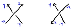
1	3	5	7	9	11	13
-8	14	-10	-2	-12	-6	4

It is just a coincidence that the first row consists only of odd numbers. In general, non-alternating knots will have the odd numbers in the first and second rows.

We can sort the vertices so that the first row is in increasing order. In this form, if we record only the second row we can reconstruct the first: it is $\{1,2,\dots ,2n\}-{\bigcup }_i\left|a_i\right|$ in sorted order, where $(a_1,\dots ,a_n)$ is the second row. If we only care about prime diagrams up to mirror image, we can remove the signs, since we know the second row is always for the overstrand.

Using a straightforward encoding scheme, the list of $n$ numbers in the range $[1,2n]$ takes $n{\log }_2\left(2n\right)$ bits to store, and the signs take an additional $n$ bits. This is the same amount of space as a signed DT code takes when stored as a list of numbers.

Of course, there are many things one could try to improve this encoding. There are $\frac{\left(2n\right)!}{n!n!}$ subsets that can appear in the first row, and for each of these there are $2^n$ sign choices and $n!$ permutations of the second row, giving $2^n\frac{\left(2n\right)!}{n!}$ possible codes. This is exactly the same as the number of Gauss codes of the same size, as one would expect, so the analysis from that section applies.

There are 1,701,936 knots up to 16 crossings, and using this simple encoding scheme (as a list of numbers) they can be stored in about 16.2 MB with either this system or unsigned DT codes. Without using the fact that prime diagrams only need a single bit to specify chirality, it would take an additional 3.2 MB to store intersection signs. A more optimal unsigned DT code scheme (using derangements) would take about 12 MB.

5. Virtual knots

A virtual knot is what happens when you start with knots, go to combinatorial map representations of diagrams, then generalize to allow all combinatorial map representations, whether or not they might be planar. Then, since Reidemeister moves can be done directly on combinatorial map representations, there is a notion of virtual knot equivalence. It is a surprising fact that if two knots are equivalent through “virtual moves,” then they are equivalent as knots^[8], so the theory doesn’t just collapse.

Something that wasn’t mentioned before was that (connected) combinatorial maps are good for representing graphs embedded in closed oriented surfaces, with the proviso that each face be a disk. And, given an arbitrary combinatorial map, the genus of a surface it can be embedded in with this condition can be computed from the number of vertices, edges, and faces: $v-e+f=2b_0-2g$, where $b_0$ is the number of connected components of the map.

Each virtual knot can be drawn on a surface this way. But, since paper tends to be planar, and since only the combinatorial map part really needs to be recorded, what we can do is draw the crossings and then connect them together without any regard for whether the edges intersect or not — only what is connected to what matters. These intersections, which are artefacts of non-planarity, are called virtual crossings. In the literature you will see “detour moves” as being part of the definition of virtual knot equivalence, but you can think of the move as being the act of erasing an edge and redrawing it with a new route. This doesn’t change the combinatorial map.

For example, here is the “virtual trefoil knot,” which is a nontrivial crossing number $2$ virtual knot that would more comfortably be drawn on a torus:

There are a number of things about encoding knots that fail for virtual knots. The first is that the intersection sign truly matters, since changing a crossing’s intersection sign (what Kauffman calls “flanking by virtuals”) gives another valid virtual knot. In the example of the virtual trefoil, changing the intersection sign of either crossing gives the unknot!

Another thing that fails is that the DT involution is no longer parity reversing, and the involution comes from the full symmetric group on $2n$ symbols.

Using the dart numbering scheme from the DT section, starting with the positive understrand, we can represent the virtual trefoil through the following combinatorial map:

3	2
-1	-4
-3	-2
1	4

With the code from the previous section, we can represent this virtual trefoil as $$-4,-1.$$

The space analysis from the previous section applies to all codes, planar or non-planar. So $20$-crossing virtual knots can be stored within $16$ bytes, too.