If ![]() is a random variable with corresponding probability density
function
is a random variable with corresponding probability density
function ![]() , then we define the expected value of
, then we define the expected value of ![]() to be
to be
We define the variance of ![]() to be
to be
As with the variance of a discrete random variable, there is a simpler formula for the variance.
![\begin{eqnarray*}
\mathrm{Var}(X) & = & \int_{-\infty}^\infty [x - E(X)] f(x) dx...
...2 \times 1 \\
& = & \int_{-\infty}^\infty x^2 f(x) dx - E(X)^2
\end{eqnarray*}](img5.png)
The expected value should be regarded as the average value. When ![]() is a
discrete random variable, then the expected value of
is a
discrete random variable, then the expected value of ![]() is precisely the mean
of the corresponding data.
is precisely the mean
of the corresponding data.
The variance should be regarded as (something like) the average of the difference of the actual values from the average. A larger variance indicates a wider spread of values.
As with discrete random variables, sometimes one uses the standard deviation,
![]() , to
measure the spread of the distribution instead.
, to
measure the spread of the distribution instead.
The uniform distribution on the interval ![]() has the
probability density function
has the
probability density function
Letting ![]() be the associated random variable, compute
be the associated random variable, compute ![]() and
and
![]() .
.
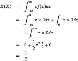
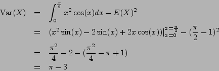
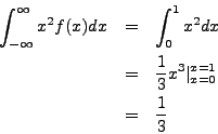
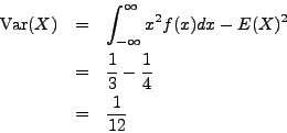
We compute
Hence,
Let ![]() be the random variable with probability density function
be the random variable with probability density function
![]() .
.
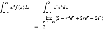
Compute ![]() and
and
![]() .
.
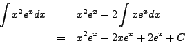
Integrating by parts with ![]() and
and ![]() , we see that
, we see that
![]() . Thus,
. Thus,
![\begin{eqnarray*}
E(X) & = & \int_{-\infty}^\infty x f(x) dx \\
& = & \int_{-\...
...\\
& = & \lim_{r \to -\infty} [-1 - r e^r + e^r] \\
& = & 1
\end{eqnarray*}](img18.png)
[We used L'Hôpital's rule to see that
![]() .]
.]
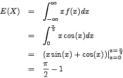
We compute
So,
This gives
![]() .
.
Suppose that the random variable ![]() has a cumulative distribution function
has a cumulative distribution function
![]()
Compute ![]() and
and
![]() .
.
First, we must find the probability density function of ![]() .
Differentiating we find that the function
.
Differentiating we find that the function
is the derivative of ![]() at all but two points. Thus,
at all but two points. Thus, ![]() is a
probability density function for
is a
probability density function for ![]() .
.
Integrating by parts, we compute